इस ब्लॉग्स का सृजन भारत वर्ष में आयोजित होने वाली समस्त प्रकार की प्रतियोगी एवं भर्ती परीक्षाओं में सभी प्रकार के प्रतिभागियों को संतुष्ठ करते हुए वांछित पाठ्य विषय वस्तु का संपादन और संगर्हण किया गया हैं , सभी विषय वस्तुए सर्वाधिकार सुरक्षित हैं ,न लाभ न हानि पर संचालित कि जा रही , इन सभी विषय वस्तुए को भारत वर्षमें हिंदी , गुजराती, मराठी , कन्नड़ , तमिल, तेलगु, बांग्ला , उर्दू, आदि में अनूदित कर के देखा जा सकता हैं , सभी को भविष्य कि हार्दिक शुभकामना सहित सुझाव सादर आमंत्रित हैं,
इस ब्लॉग्स को सृजन करने में आप सभी से सादर सुझाव आमंत्रित हैं , कृपया अपने सुझाव और प्रविष्टियाँ प्रेषित करे , इसका संपूर्ण कार्य क्षेत्र विश्व ज्ञान समुदाय हैं , जो सभी प्रतियोगियों के कॅरिअर निर्माण महत्त्वपूर्ण योगदान देगा ,आप अपने सुझाव इस मेल पत्ते पर भेज सकते हैं - chandrashekhar.malav@yahoo.com
DBMS-DATABASE MANAGEMENT SYSTEMS
DBMS - Overview
Database is collection of data which is related by some aspect. Data is collection of facts and figures which can be processed to produce information. Name of a student, age, class and her subjects can be counted as data for recording purposes.
Mostly data represents recordable facts. Data aids in producing information which is based on facts. For example, if we have data about marks obtained by all students, we can then conclude about toppers and average marks etc.
A database management system stores data, in such a way which is easier to retrieve, manipulate and helps to produce information.
Characteristics
Traditionally data was organized in file formats. DBMS was all new concepts then and all the research was done to make it to overcome all the deficiencies in traditional style of data management. Modern DBMS has the following characteristics:
Real-world entity: Modern DBMS are more realistic and uses real world entities to design its architecture. It uses the behavior and attributes too. For example, a school database may use student as entity and their age as their attribute.
Relation-based tables: DBMS allows entities and relations among them to form as tables. This eases the concept of data saving. A user can understand the architecture of database just by looking at table names etc.
Isolation of data and application: A database system is entirely different than its data. Where database is said to active entity, data is said to be passive one on which the database works and organizes. DBMS also stores metadata which is data about data, to ease its own process.
Less redundancy: DBMS follows rules of normalization, which splits a relation when any of its attributes is having redundancy in values. Following normalization, which itself is a mathematically rich and scientific process, make the entire database to contain as less redundancy as possible.
Consistency: DBMS always enjoy the state on consistency where the previous form of data storing applications like file processing does not guarantee this. Consistency is a state where every relation in database remains consistent. There exist methods and techniques, which can detect attempt of leaving database in inconsistent state.
Query Language: DBMS is equipped with query language, which makes it more efficient to retrieve and manipulate data. A user can apply as many and different filtering options, as he or she wants. Traditionally it was not possible where file-processing system was used.
ACID Properties: DBMS follows the concepts for ACID properties, which stands for Atomicity, Consistency, Isolation and Durability. These concepts are applied on transactions, which manipulate data in database. ACID properties maintains database in healthy state in multi-transactional environment and in case of failure.
Multiuser and Concurrent Access: DBMS support multi-user environment and allows them to access and manipulate data in parallel. Though there are restrictions on transactions when they attempt to handle same data item, but users are always unaware of them.
Multiple views: DBMS offers multiples views for different users. A user who is in sales department will have a different view of database than a person working in production department. This enables user to have a concentrate view of database according to their requirements.
Security: Features like multiple views offers security at some extent where users are unable to access data of other users and departments. DBMS offers methods to impose constraints while entering data into database and retrieving data at later stage. DBMS offers many different levels of security features, which enables multiple users to have different view with different features. For example, a user in sales department cannot see data of purchase department is one thing, additionally how much data of sales department he can see, can also be managed. Because DBMS is not saved on disk as traditional file system it is very hard for a thief to break the code.
Users
DBMS is used by various users for various purposes. Some may involve in retrieving data and some may involve in backing it up. Some of them are described as follows:
[Image: DBMS Users]
Administrators: A bunch of users maintain the DBMS and are responsible for administrating the database. They are responsible to look after its usage and by whom it should be used. They create users access and apply limitation to maintain isolation and force security. Administrators also look after DBMS resources like system license, software application and tools required and other hardware related maintenance.
Designer: This is the group of people who actually works on designing part of database. The actual database is started with requirement analysis followed by a good designing process. They people keep a close watch on what data should be kept and in what format. They identify and design the whole set of entities, relations, constraints and views.
End Users: This group contains the persons who actually take advantage of database system. End users can be just viewers who pay attention to the logs or market rates or end users can be as sophisticated as business analysts who takes the most of it.
DBMS - Architecture
The design of a Database Management System highly depends on its architecture. It can be centralized or decentralized or hierarchical. DBMS architecture can be seen as single tier or multi tier. n-tier architecture divides the whole system into related but independent n modules, which can be independently modified, altered, changed or replaced.
In 1-tier architecture, DBMS is the only entity where user directly sits on DBMS and uses it. Any changes done here will directly be done on DBMS itself. It does not provide handy tools for end users and preferably database designer and programmers use single tier architecture.
If the architecture of DBMS is 2-tier then must have some application, which uses the DBMS. Programmers use 2-tier architecture where they access DBMS by means of application. Here application tier is entirely independent of database in term of operation, design and programming.
3-tier architecture
Most widely used architecture is 3-tier architecture. 3-tier architecture separates it tier from each other on basis of users. It is described as follows:
[Image: 3-tier DBMS architecture]
Database (Data) Tier: At this tier, only database resides. Database along with its query processing languages sits in layer-3 of 3-tier architecture. It also contains all relations and their constraints.
Application (Middle) Tier: At this tier the application server and program, which access database, resides. For a user this application tier works as abstracted view of database. Users are unaware of any existence of database beyond application. For database-tier, application tier is the user of it. Database tier is not aware of any other user beyond application tier. This tier works as mediator between the two.
User (Presentation) Tier: An end user sits on this tier. From a users aspect this tier is everything. He/she doesn't know about any existence or form of database beyond this layer. At this layer multiple views of database can be provided by the application. All views are generated by applications, which resides in application tier.
Multiple tier database architecture is highly modifiable as almost all its components are independent and can be changed independently.<
DBMS - Data Models
Data model tells how the logical structure of a database is modeled. Data Models are fundamental entities to introduce abstraction in DBMS. Data models define how data is connected to each other and how it will be processed and stored inside the system.
The very first data model could be flat data-models where all the data used to be kept in same plane. Because earlier data models were not so scientific they were prone to introduce lots of duplication and update anomalies.
Entity-Relationship Model
Entity-Relationship model is based on the notion of real world entities and relationship among them. While formulating real-world scenario into database model, ER Model creates entity set, relationship set, general attributes and constraints.
ER Model is best used for the conceptual design of database.
ER Model is based on:
Entities and their attributes
Relationships among entities
These concepts are explained below.
[Image: ER Model]
Entity
An entity in ER Model is real world entity, which has some properties called attributes. Every attribute is defined by its set of values, called domain.
For example, in a school database, a student is considered as an entity. Student has various attributes like name, age and class etc.
Relationship
The logical association among entities is called relationship. Relationships are mapped with entities in various ways. Mapping cardinalities define the number of association between two entities.
The most popular data model in DBMS is Relational Model. It is more scientific model then others. This model is based on first-order predicate logic and defines table as an n-ary relation.
[Image: Table in relational Model]
The main highlights of this model are:
Data is stored in tables called relations.
Relations can be normalized.
In normalized relations, values saved are atomic values.
Each row in relation contains unique value
Each column in relation contains values from a same domain.
Database schema skeleton structure of and it represents the logical view of entire database. It tells about how the data is organized and how relation among them is associated. It formulates all database constraints that would be put on data in relations, which resides in database.
A database schema defines its entities and the relationship among them. Database schema is a descriptive detail of the database, which can be depicted by means of schema diagrams. All these activities are done by database designer to help programmers in order to give some ease of understanding all aspect of database.
[Image: Database Schemas]
Database schema can be divided broadly in two categories:
Physical Database Schema: This schema pertains to the actual storage of data and its form of storage like files, indices etc. It defines the how data will be stored in secondary storage etc.
Logical Database Schema: This defines all logical constraints that need to be applied on data stored. It defines tables, views and integrity constraints etc.
Database Instance
It is important that we distinguish these two terms individually. Database schema is the skeleton of database. It is designed when database doesn't exist at all and very hard to do any changes once the database is operational. Database schema does not contain any data or information.
Database instances, is a state of operational database with data at any given time. This is a snapshot of database. Database instances tend to change with time. DBMS ensures that its every instance (state) must be a valid state by keeping up to all validation, constraints and condition that database designers has imposed or it is expected from DBMS itself.
DBMS - Data Independence
If the database system is not multi-layered then it will be very hard to make any changes in the database system. Database systems are designed in multi-layers as we leant earlier.
Data Independence:
There's a lot of data in whole database management system other than user's data. DBMS comprises of three kinds of schemas, which is in turn data about data (Meta-Data). Meta-data is also stored along with database, which once stored is then hard to modify. But as DBMS expands, it needs to be changed over the time satisfy the requirements of users. But if the whole data were highly dependent it would become tedious and highly complex.
[Image: Data independence]
Data about data itself is divided in layered architecture so that when we change data at one layer it does not affect the data layered at different level. This data is independent but mapped on each other.
Logical Data Independence
Logical data is data about database, that is, it stores information about how data is managed inside. For example, a table (relation) stored in the database and all constraints, which are applied on that relation.
Logical data independence is a kind of mechanism, which liberalizes itself from actual data stored on the disk. If we do some changes on table format it should not change the data residing on disk.
Physical Data Independence
All schemas are logical and actual data is stored in bit format on the disk. Physical data independence is the power to change the physical data without impacting the schema or logical data.
For example, in case we want to change or upgrade the storage system itself, that is, using SSD instead of Hard-disks should not have any impact on logical data or schemas.
ER Model Basic Concepts
Entity relationship model defines the conceptual view of database. It works around real world entity and association among them. At view level, ER model is considered well for designing databases.
Entity
A real-world thing either animate or inanimate that can be easily identifiable and distinguishable. For example, in a school database, student, teachers, class and course offered can be considered as entities. All entities have some attributes or properties that give them their identity.
An entity set is a collection of similar types of entities. Entity set may contain entities with attribute sharing similar values. For example, Students set may contain all the student of a school; likewise Teachers set may contain all the teachers of school from all faculties. Entities sets need not to be disjoint.
Attributes
Entities are represented by means of their properties, called attributes. All attributes have values. For example, a student entity may have name, class, age as attributes.
There exist a domain or range of values that can be assigned to attributes. For example, a student's name cannot be a numeric value. It has to be alphabetic. A student's age cannot be negative, etc.
TYPES OF ATTRIBUTES:
Simple attribute:
Simple attributes are atomic values, which cannot be divided further. For example, student's phone-number is an atomic value of 10 digits.
Composite attribute:
Composite attributes are made of more than one simple attribute. For example, a student's complete name may have first_name and last_name.
Derived attribute:
Derived attributes are attributes, which do not exist physical in the database, but there values are derived from other attributes presented in the database. For example, average_salary in a department should be saved in database instead it can be derived. For another example, age can be derived from data_of_birth.
Single-valued attribute:
Single valued attributes contain on single value. For example: Social_Security_Number.
Multi-value attribute:
Multi-value attribute may contain more than one values. For example, a person can have more than one phone numbers, email_addresses etc.
These attribute types can come together in a way like:
simple single-valued attributes
simple multi-valued attributes
composite single-valued attributes
composite multi-valued attributes
ENTITY-SET AND KEYS
Key is an attribute or collection of attributes that uniquely identifies an entity among entity set.
For example, roll_number of a student makes her/him identifiable among students.
Super Key: Set of attributes (one or more) that collectively identifies an entity in an entity set.
Candidate Key: Minimal super key is called candidate key that is, supers keys for which no proper subset are a superkey. An entity set may have more than one candidate key.
Primary Key: This is one of the candidate key chosen by the database designer to uniquely identify the entity set.
Relationship
The association among entities is called relationship. For example, employee entity has relation works_at with department. Another example is for student who enrolls in some course. Here, Works_at and Enrolls are called relationship.
RELATIONSHIP SET:
Relationship of similar type is called relationship set. Like entities, a relationship too can have attributes. These attributes are called descriptive attributes.
DEGREE OF RELATIONSHIP
The number of participating entities in an relationship defines the degree of the relationship.
Binary = degree 2
Ternary = degree 3
n-ary = degree
MAPPING CARDINALITIES:
Cardinality defines the number of entities in one entity set which can be associated to the number of entities of other set via relationship set.
One-to-one: one entity from entity set A can be associated with at most one entity of entity set B and vice versa.
[Image: One-to-one relation]
One-to-many: One entity from entity set A can be associated with more than one entities of entity set B but from entity set B one entity can be associated with at most one entity.
[Image: One-to-many relation]
Many-to-one: More than one entities from entity set A can be associated with at most one entity of entity set B but one entity from entity set B can be associated with more than one entity from entity set A.
[Image: Many-to-one relation]
Many-to-many: one entity from A can be associated with more than one entity from B and vice versa.
[Image: Many-to-many relation]
ER Diagram Representation
Now we shall learn how ER Model is represented by means of ER diagram. Every object like entity, attributes of an entity, relationship set, and attributes of relationship set can be represented by tools of ER diagram.
Entity
Entities are represented by means of rectangles. Rectangles are named with the entity set they represent.
[Image: Entities in a school database]
Attributes
Attributes are properties of entities. Attributes are represented by means of eclipses. Every eclipse represents one attribute and is directly connected to its entity (rectangle).
[Image: Simple Attributes]
If the attributes are composite, they are further divided in a tree like structure. Every node is then connected to its attribute. That is composite attributes are represented by eclipses that are connected with an eclipse.
[Image: Composite Attributes]
Multivalued attributes are depicted by double eclipse.
[Image: Multivalued Attributes]
Derived attributes are depicted by dashed eclipse.
[Image: Derived Attributes]
Relationship
Relationships are represented by diamond shaped box. Name of the relationship is written in the diamond-box. All entities (rectangles), participating in relationship, are connected to it by a line.
BINARY RELATIONSHIP AND CARDINALITY
A relationship where two entities are participating, is called a binary relationship. Cardinality is the number of instance of an entity from a relation that can be associated with the relation.
One-to-one
When only one instance of entity is associated with the relationship, it is marked as '1'. This image below reflects that only 1 instance of each entity should be associated with the relationship. It depicts one-to-one relationship
[Image: One-to-one]
One-to-many
When more than one instance of entity is associated with the relationship, it is marked as 'N'. This image below reflects that only 1 instance of entity on the left and more than one instance of entity on the right can be associated with the relationship. It depicts one-to-many relationship
[Image: One-to-many]
Many-to-one
When more than one instance of entity is associated with the relationship, it is marked as 'N'. This image below reflects that more than one instance of entity on the left and only one instance of entity on the right can be associated with the relationship. It depicts many-to-one relationship
[Image: Many-to-one]
Many-to-many
This image below reflects that more than one instance of entity on the left and more than one instance of entity on the right can be associated with the relationship. It depicts many-to-many relationship
[Image: Many-to-many]
PARTICIPATION CONSTRAINTS
Total Participation: Each entity in the entity is involved in the relationship. Total participation is represented by double lines.
Partial participation: Not all entities are involved in the relation ship. Partial participation is represented by single line.
[Image: Participation Constraints]
Generalization, Aggregation
ER Model has the power of expressing database entities in conceptual hierarchical manner such that, as the hierarchical goes up it generalize the view of entities and as we go deep in the hierarchy it gives us detail of every entity included.
Going up in this structure is called generalization, where entities are clubbed together to represent a more generalized view. For example, a particular student named, Mira can be generalized along with all the students, the entity shall be student, and further a student is person. The reverse is called specialization where a person is student, and that student is Mira.
Generalization
As mentioned above, the process of generalizing entities, where the generalized entities contain the properties of all the generalized entities is called Generalization. In generalization, a number of entities are brought together into one generalized entity based on their similar characteristics. For an example, pigeon, house sparrow, crow and dove all can be generalized as Birds.
[Image: Generalization]
Specialization
Specialization is a process, which is opposite to generalization, as mentioned above. In specialization, a group of entities is divided into sub-groups based on their characteristics. Take a group Person for example. A person has name, date of birth, gender etc. These properties are common in all persons, human beings. But in a company, a person can be identified as employee, employer, customer or vendor based on what role do they play in company.
[Image: Specialization]
Similarly, in a school database, a person can be specialized as teacher, student or staff; based on what role do they play in school as entities.
Inheritance
We use all above features of ER-Model, in order to create classes of objects in object oriented programming. This makes it easier for the programmer to concentrate on what she is programming. Details of entities are generally hidden from the user, this process known as abstraction.
One of the important features of Generalization and Specialization, is inheritance, that is, the attributes of higher-level entities are inherited by the lower level entities.
[Image: Inheritance]
For example, attributes of a person like name, age, and gender can be inherited by lower level entities like student and teacher etc.
DBMS Codd's Rules
Dr Edgar F. Codd did some extensive research in Relational Model of database systems and came up with twelve rules of his own which according to him, a database must obey in order to be a true relational database.
These rules can be applied on a database system that is capable of managing is stored data using only its relational capabilities. This is a foundation rule, which provides a base to imply other rules on it.
Rule 1: Information rule
This rule states that all information (data), which is stored in the database, must be a value of some table cell. Everything in a database must be stored in table formats. This information can be user data or meta-data.
Rule 2: Guaranteed Access rule
This rule states that every single data element (value) is guaranteed to be accessible logically with combination of table-name, primary-key (row value) and attribute-name (column value). No other means, such as pointers, can be used to access data.
Rule 3: Systematic Treatment of NULL values
This rule states the NULL values in the database must be given a systematic treatment. As a NULL may have several meanings, i.e. NULL can be interpreted as one the following: data is missing, data is not known, data is not applicable etc.
Rule 4: Active online catalog
This rule states that the structure description of whole database must be stored in an online catalog, i.e. data dictionary, which can be accessed by the authorized users. Users can use the same query language to access the catalog which they use to access the database itself.
Rule 5: Comprehensive data sub-language rule
This rule states that a database must have a support for a language which has linear syntax which is capable of data definition, data manipulation and transaction management operations. Database can be accessed by means of this language only, either directly or by means of some application. If the database can be accessed or manipulated in some way without any help of this language, it is then a violation.
Rule 6: View updating rule
This rule states that all views of database, which can theoretically be updated, must also be updatable by the system.
Rule 7: High-level insert, update and delete rule
This rule states the database must employ support high-level insertion, updation and deletion. This must not be limited to a single row that is, it must also support union, intersection and minus operations to yield sets of data records.
Rule 8: Physical data independence
This rule states that the application should not have any concern about how the data is physically stored. Also, any change in its physical structure must not have any impact on application.
Rule 9: Logical data independence
This rule states that the logical data must be independent of its user’s view (application). Any change in logical data must not imply any change in the application using it. For example, if two tables are merged or one is split into two different tables, there should be no impact the change on user application. This is one of the most difficult rule to apply.
Rule 10: Integrity independence
This rule states that the database must be independent of the application using it. All its integrity constraints can be independently modified without the need of any change in the application. This rule makes database independent of the front-end application and its interface.
Rule 11: Distribution independence
This rule states that the end user must not be able to see that the data is distributed over various locations. User must also see that data is located at one site only. This rule has been proven as a foundation of distributed database systems.
Rule 12: Non-subversion rule
This rule states that if a system has an interface that provides access to low level records, this interface then must not be able to subvert the system and bypass security and integrity constraints.
Relational Data Model
Relational data model is the primary data model, which is used widely around the world for data storage and processing. This model is simple and have all the properties and capabilities required to process data with storage efficiency.
Concepts
Tables: In relation data model, relations are saved in the format of Tables. This format stores the relation among entities. A table has rows and columns, where rows represent records and columns represents the attributes.
Tuple: A single row of a table, which contains a single record for that relation is called a tuple.
Relation instance: A finite set of tuples in the relational database system represents relation instance. Relation instances do not have duplicate tuples.
Relation schema: This describes the relation name (table name), attributes and their names.
Relation key: Each row has one or more attributes which can identify the row in the relation (table) uniquely, is called the relation key.
Attribute domain: Every attribute has some pre-defined value scope, known as attribute domain.
Constraints
Every relation has some conditions that must hold for it to be a valid relation. These conditions are called Relational Integrity Constraints. There are three main integrity constraints.
Key Constraints
Domain constraints
Referential integrity constraints
KEY CONSTRAINTS:
There must be at least one minimal subset of attributes in the relation, which can identify a tuple uniquely. This minimal subset of attributes is called key for that relation. If there are more than one such minimal subsets, these are called candidate keys.
Key constraints forces that:
in a relation with a key attribute, no two tuples can have identical value for key attributes.
key attribute can not have NULL values.
Key constrains are also referred to as Entity Constraints.
DOMAIN CONSTRAINTS
Attributes have specific values in real-world scenario. For example, age can only be positive integer. The same constraints has been tried to employ on the attributes of a relation. Every attribute is bound to have a specific range of values. For example, age can not be less than zero and telephone number can not be a outside 0-9.
REFERENTIAL INTEGRITY CONSTRAINTS
This integrity constraints works on the concept of Foreign Key. A key attribute of a relation can be referred in other relation, where it is called foreign key.
Referential integrity constraint states that if a relation refers to an key attribute of a different or same relation, that key element must exists.
Relational Algebra
Relational database systems are expected to be equipped by a query language that can assist its user to query the database instances. This way its user empowers itself and can populate the results as required. There are two kinds of query languages, relational algebra and relational calculus.
Relational algebra
Relational algebra is a procedural query language, which takes instances of relations as input and yields instances of relations as output. It uses operators to perform queries. An operator can be either unary or binary. They accept relations as their input and yields relations as their output. Relational algebra is performed recursively on a relation and intermediate results are also considered relations.
Fundamental operations of Relational algebra:
Select
Project
Union
Set different
Cartesian product
Rename
These are defined briefly as follows:
Select Operation (σ)
Selects tuples that satisfy the given predicate from a relation.
Notation σp(r)
Where p stands for selection predicate and r stands for relation. p is prepositional logic formulae which may use connectors like and, or and not. These terms may use relational operators like: =, ≠, ≥, < , >, ≤.
For example:
σsubject="database"(Books)
Output : Selects tuples from books where subject is 'database'.
σsubject="database"and price="450"(Books)
Output : Selects tuples from books where subject is 'database' and 'price' is 450.
σsubject="database"and price <"450"or year >"2010"(Books)
Output : Selects tuples from books where subject is 'database' and 'price' is 450 or the publication year is greater than 2010, that is published after 2010.
Project Operation (∏)
Projects column(s) that satisfy given predicate.
Notation: ∏A1, A2, An (r)
Where a1, a2 , an are attribute names of relation r.
Duplicate rows are automatically eliminated, as relation is a set.
for example:
∏subject, author(Books)
Selects and projects columns named as subject and author from relation Books.
Union Operation (∪)
Union operation performs binary union between two given relations and is defined as:
r ∪ s ={ t | t ∈ r or t ∈ s}
Notion: r U s
Where r and s are either database relations or relation result set (temporary relation).
For a union operation to be valid, the following conditions must hold:
r, s must have same number of attributes.
Attribute domains must be compatible.
Duplicate tuples are automatically eliminated.
∏author(Books)∪∏author(Articles)
Output : Projects the name of author who has either written a book or an article or both.
Set Difference ( − )
The result of set difference operation is tuples which present in one relation but are not in the second relation.
Notation: r − s
Finds all tuples that are present in r but not s.
∏author(Books)−∏author(Articles)
Output: Results the name of authors who has written books but not articles.
Cartesian Product (Χ)
Combines information of two different relations into one.
Notation: r Χ s
Where r and s are relations and there output will be defined as:
r Χ s = { q t | q ∈ r and t ∈ s}
∏author ='tutorialspoint'(BooksΧArticles)
Output : yields a relation as result which shows all books and articles written by tutorialspoint.
Rename operation ( ρ )
Results of relational algebra are also relations but without any name. The rename operation allows us to rename the output relation. rename operation is denoted with small greek letter rho ρ
Notation: ρx (E)
Where the result of expression E is saved with name of x.
Additional operations are:
Set intersection
Assignment
Natural join
Relational Calculus
In contrast with Relational Algebra, Relational Calculus is non-procedural query language, that is, it tells what to do but never explains the way, how to do it.
Relational calculus exists in two forms:
Tuple relational calculus (TRC)
Filtering variable ranges over tuples
Notation: { T | Condition }
Returns all tuples T that satisfies condition.
For Example:
{ T.name |Author(T) AND T.article ='database'}
Output: returns tuples with 'name' from Author who has written article on 'database'.
TRC can be quantified also. We can use Existential ( ∃ )and Universal Quantifiers ( ∀ ).
For example:
{ R|∃T ∈Authors(T.article='database' AND R.name=T.name)}
Output : the query will yield the same result as the previous one.
Domain relational calculus (DRC)
In DRC the filtering variable uses domain of attributes instead of entire tuple values (as done in TRC, mentioned above).
Notation:
{ a1, a2, a3, ..., an | P (a1, a2, a3, ... ,an)}
where a1, a2 are attributes and P stands for formulae built by inner attributes.
For example:
{< article, page, subject >|
∈TutorialsPoint∧ subject ='database'}
Output: Yields Article, Page and Subject from relation TutorialsPoint where Subject is database.
Just like TRC, DRC also can be written using existential and universal quantifiers. DRC also involves relational operators.
Expression power of Tuple relation calculus and Domain relation calculus is equivalent to Relational Algebra.
ER to Relational Model
ER Model when conceptualized into diagrams gives a good overview of entity-relationship, which is easier to understand. ER diagrams can be mapped to Relational schema that is, it is possible to create relational schema using ER diagram. Though we cannot import all the ER constraints into Relational model but an approximate schema can be generated.
There are more than one processes and algorithms available to convert ER Diagrams into Relational Schema. Some of them are automated and some of them are manual process. We may focus here on the mapping diagram contents to relational basics.
ER Diagrams mainly comprised of:
Entity and its attributes
Relationship, which is association among entities.
Mapping Entity
An entity is a real world object with some attributes.
Mapping Process (Algorithm):
[Image: Mapping Entity]
Create table for each entity
Entity's attributes should become fields of tables with their respective data types.
Declare primary key
Mapping relationship
A relationship is association among entities.
Mapping process (Algorithm):
[Image: Mapping relationship]
Create table for a relationship
Add the primary keys of all participating Entities as fields of table with their respective data types.
If relationship has any attribute, add each attribute as field of table.
Declare a primary key composing all the primary keys of participating entities.
Declare all foreign key constraints.
Mapping Weak Entity Sets
A weak entity sets is one which does not have any primary key associated with it.
Mapping process (Algorithm):
[Image: Mapping Weak Entity Sets]
Create table for weak entity set
Add all its attributes to table as field
Add the primary key of identifying entity set
Declare all foreign key constraints
Mapping hierarchical entities
ER specialization or generalization comes in the form of hierarchical entity sets.
Mapping process (Algorithm):
[Image: Mapping hierarchical entities]
Create tables for all higher level entities
Create tables for lower level entities
Add primary keys of higher level entities in the table of lower level entities
In lower level tables, add all other attributes of lower entities.
Declare primary key of higher level table the primary key for lower level table
Declare foreign key constraints.
SQL Overview
SQL is a programming language for Relational Databases. It is designed over relational algebra and tuple relational calculus. SQL comes as a package with all major distributions of RDBMS.
SQL comprises both data definition and data manipulation languages. Using the data definition properties of SQL, one can design and modify database schema whereas data manipulation properties allows SQL to store and retrieve data from database.
Data definition Language
SQL uses the following set of commands to define database schema:
CREATE
Creates new databases, tables and views from RDBMS
For example:
Create database tutorialspoint;
Create table article;
Create view for_students;
DROP
Drop commands deletes views, tables and databases from RDBMS
Drop object_type object_name;
Drop database tutorialspoint;
Drop table article;
Drop view for_students;
ALTER
Modifies database schema.
Alter object_type object_name parameters;
for example:
Alter table article add subject varchar;
This command adds an attribute in relation article with name subject of string type.
Data Manipulation Language
SQL is equipped with data manipulation language. DML modifies the database instance by inserting, updating and deleting its data. DML is responsible for all data modification in databases. SQL contains the following set of command in DML section:
SELECT/FROM/WHERE
INSERT INTO/VALUES
UPDATE/SET/WHERE
DELETE FROM/WHERE
These basic constructs allows database programmers and users to enter data and information into the database and retrieve efficiently using a number of filter options.
SELECT/FROM/WHERE
SELECT
This is one of the fundamental query command of SQL. It is similar to projection operation of relational algebra. It selects the attributes based on the condition described by WHERE clause.
FROM
This clause takes a relation name as an argument from which attributes are to be selected/projected. In case more than one relation names are given this clause corresponds to cartesian product.
WHERE
This clause defines predicate or conditions which must match in order to qualify the attributes to be projected.
For example:
Select author_name
From book_author
Where age >50;
This command will project names of author’s from book_author relation whose age is greater than 50.
INSERT INTO/VALUES
This command is used for inserting values into rows of table (relation).
INSERT INTO tutorialspoint (Author,Subject) VALUES ("anonymous","computers");
UPDATE/SET/WHERE
This command is used for updating or modifying values of columns of table (relation).
Syntax is
UPDATE table_name SET column_name = value [, column_name = value ...][WHERE condition]
For example:
UPDATE tutorialspoint SET Author="webmaster" WHERE Author="anonymous";
DELETE/FROM/WHERE
This command is used for removing one or more rows from table (relation).
Syntax is
DELETE FROM table_name [WHERE condition];
For example:
DELETE FROM tutorialspoints
  WHERE Author="unknown";
For in-depth and practical knowledge of SQL, click here.
Database Normalization
Functional Dependency
Functional dependency (FD) is set of constraints between two attributes in a relation. Functional dependency says that if two tuples have same values for attributes A1, A2,..., An then those two tuples must have to have same values for attributes B1, B2, ..., Bn.
Functional dependency is represented by arrow sign (→), that is X→Y, where X functionally determines Y. The left hand side attributes determines the values of attributes at right hand side.
Armstrong's Axioms
If F is set of functional dependencies then the closure of F, denoted as F+, is the set of all functional dependencies logically implied by F. Armstrong's Axioms are set of rules, when applied repeatedly generates closure of functional dependencies.
Reflexive rule: If alpha is a set of attributes and beta is_subset_of alpha, then alpha holds beta.
Augmentation rule: if a → b holds and y is attribute set, then ay → by also holds. That is adding attributes in dependencies, does not change the basic dependencies.
Transitivity rule: Same as transitive rule in algebra, if a → b holds and b → c holds then a → c also hold. a → b is called as a functionally determines b.
Trivial Functional Dependency
Trivial: If an FD X → Y holds where Y subset of X, then it is called a trivial FD. Trivial FDs are always hold.
Non-trivial: If an FD X → Y holds where Y is not subset of X, then it is called non-trivial FD.
Completely non-trivial: If an FD X → Y holds where x intersect Y = Φ, is said to be completely non-trivial FD.
Normalization
If a database design is not perfect it may contain anomalies, which are like a bad dream for database itself. Managing a database with anomalies is next to impossible.
Update anomalies: if data items are scattered and are not linked to each other properly, then there may be instances when we try to update one data item that has copies of it scattered at several places, few instances of it get updated properly while few are left with there old values. This leaves database in an inconsistent state.
Deletion anomalies: we tried to delete a record, but parts of it left undeleted because of unawareness, the data is also saved somewhere else.
Insert anomalies: we tried to insert data in a record that does not exist at all.
Normalization is a method to remove all these anomalies and bring database to consistent state and free from any kinds of anomalies.
First Normal Form:
This is defined in the definition of relations (tables) itself. This rule defines that all the attributes in a relation must have atomic domains. Values in atomic domain are indivisible units.
[Image: Unorganized relation]
We re-arrange the relation (table) as below, to convert it to First Normal Form
[Image: Relation in 1NF]
Each attribute must contain only single value from its pre-defined domain.
Second Normal Form:
Before we learn about second normal form, we need to understand the following:
Prime attribute: an attribute, which is part of prime-key, is prime attribute.
Non-prime attribute: an attribute, which is not a part of prime-key, is said to be a non-prime attribute.
Second normal form says, that every non-prime attribute should be fully functionally dependent on prime key attribute. That is, if X → A holds, then there should not be any proper subset Y of X, for that Y → A also holds.
[Image: Relation not in 2NF]
We see here in Student_Project relation that the prime key attributes are Stu_ID and Proj_ID. According to the rule, non-key attributes, i.e. Stu_Name and Proj_Name must be dependent upon both and not on any of the prime key attribute individually. But we find that Stu_Name can be identified by Stu_ID and Proj_Name can be identified by Proj_ID independently. This is called partial dependency, which is not allowed in Second Normal Form.
[Image: Relation in 2NF]
We broke the relation in two as depicted in the above picture. So there exists no partial dependency.
Third Normal Form:
For a relation to be in Third Normal Form, it must be in Second Normal form and the following must satisfy:
No non-prime attribute is transitively dependent on prime key attribute
For any non-trivial functional dependency, X → A, then either
X is a superkey or,
A is prime attribute.
[Image: Relation not in 3NF]
We find that in above depicted Student_detail relation, Stu_ID is key and only prime key attribute. We find that City can be identified by Stu_ID as well as Zip itself. Neither Zip is a superkey nor City is a prime attribute. Additionally, Stu_ID → Zip → City, so there exists transitive dependency.
[Image: Relation in 3NF]
We broke the relation as above depicted two relations to bring it into 3NF.
Boyce-Codd Normal Form:
BCNF is an extension of Third Normal Form in strict way. BCNF states that
For any non-trivial functional dependency, X → A, then X must be a super-key.
In the above depicted picture, Stu_ID is super-key in Student_Detail relation and Zip is super-key in ZipCodes relation. So,
Stu_ID → Stu_Name, Zip
And
Zip → City
Confirms, that both relations are in BCNF.
Database Joins
We understand the benefits of Cartesian product of two relation, which gives us all the possible tuples that are paired together. But Cartesian product might not be feasible for huge relations where number of tuples are in thousands and the attributes of both relations are considerable large.
Join is combination of Cartesian product followed by selection process. Join operation pairs two tuples from different relations if and only if the given join condition is satisfied.
Following section should describe briefly about join types:
Theta (θ) join
θ in Theta join is the join condition. Theta joins combines tuples from different relations provided they satisfy the theta condition.
Notation:
R1 ⋈θ R2
R1 and R2 are relations with their attributes (A1, A2, .., An ) and (B1, B2,.. ,Bn) such that no attribute matches that is R1 ∩ R2 = Φ Here θ is condition in form of set of conditions C.
Theta join can use all kinds of comparison operators.
Student
SID
Name
Std
101
Alex
10
102
Maria
11
[Table: Student Relation]
Subjects
Class
Subject
10
Math
10
English
11
Music
11
Sports
[Table: Subjects Relation]
Student_Detail =
STUDENT ⋈Student.Std=Subject.Class SUBJECT
Student_detail
SID
Name
Std
Class
Subject
101
Alex
10
10
Math
101
Alex
10
10
English
102
Maria
11
11
Music
102
Maria
11
11
Sports
[Table: Output of theta join]
Equi-Join
When Theta join uses only equality comparison operator it is said to be Equi-Join. The above example conrresponds to equi-join
Natural Join ( ⋈ )
Natural join does not use any comparison operator. It does not concatenate the way Cartesian product does. Instead, Natural Join can only be performed if the there is at least one common attribute exists between relation. Those attributes must have same name and domain.
Natural join acts on those matching attributes where the values of attributes in both relation is same.
Courses
CID
Course
Dept
CS01
Database
CS
ME01
Mechanics
ME
EE01
Electronics
EE
[Table: Relation Courses]
HoD
Dept
Head
CS
Alex
ME
Maya
EE
Mira
[Table: Relation HoD]
Courses ⋈ HoD
Dept
CID
Course
Head
CS
CS01
Database
Alex
ME
ME01
Mechanics
Maya
EE
EE01
Electronics
Mira
[Table: Relation Courses ⋈ HoD]
Outer Joins
All joins mentioned above, that is Theta Join, Equi Join and Natural Join are called inner-joins. An inner-join process includes only tuples with matching attributes, rest are discarded in resulting relation. There exists methods by which all tuples of any relation are included in the resulting relation.
There are three kinds of outer joins:
Left outer join ( R S )
All tuples of Left relation, R, are included in the resulting relation and if there exists tuples in R without any matching tuple in S then the S-attributes of resulting relation are made NULL.
Left
A
B
100
Database
101
Mechanics
102
Electronics
[Table: Left Relation]
Right
A
B
100
Alex
102
Maya
104
Mira
[Table: Right Relation]
Courses HoD
A
B
C
D
100
Database
100
Alex
101
Mechanics
---
---
102
Electronics
102
Maya
[Table: Left outer join output]
Right outer join: ( R S )
All tuples of the Right relation, S, are included in the resulting relation and if there exists tuples in S without any matching tuple in R then the R-attributes of resulting relation are made NULL.
Courses HoD
A
B
C
D
100
Database
100
Alex
102
Electronics
102
Maya
---
---
104
Mira
[Table: Right outer join output]
Full outer join: ( R S)
All tuples of both participating relations are included in the resulting relation and if there no matching tuples for both relations, their respective unmatched attributes are made NULL.
Courses HoD
A
B
C
D
100
Database
100
Alex
101
Mechanics
---
---
102
Electronics
102
Maya
---
---
104
Mira
[Table: Full outer join output]
DBMS - Storage System
Databases are stored in file formats, which contains records. At physical level, actual data is stored in electromagnetic format on some device capable of storing it for a longer amount of time. These storage devices can be broadly categorized in three types:
[Image: Memory Types]
Primary Storage: The memory storage, which is directly accessible by the CPU, comes under this category. CPU's internal memory (registers), fast memory (cache) and main memory (RAM) are directly accessible to CPU as they all are placed on the motherboard or CPU chipset. This storage is typically very small, ultra fast and volatile. This storage needs continuous power supply in order to maintain its state, i.e. in case of power failure all data are lost.
Secondary Storage: The need to store data for longer amount of time and to retain it even after the power supply is interrupted gave birth to secondary data storage. All memory devices, which are not part of CPU chipset or motherboard comes under this category. Broadly, magnetic disks, all optical disks (DVD, CD etc.), flash drives and magnetic tapes are not directly accessible by the CPU. Hard disk drives, which contain the operating system and generally not removed from the computers are, considered secondary storage and all other are called tertiary storage.
Tertiary Storage: Third level in memory hierarchy is called tertiary storage. This is used to store huge amount of data. Because this storage is external to the computer system, it is the slowest in speed. These storage devices are mostly used to backup the entire system. Optical disk and magnetic tapes are widely used storage devices as tertiary storage.
Memory Hierarchy
A computer system has well-defined hierarchy of memory. CPU has inbuilt registers, which saves data being operated on. Computer system has main memory, which is also directly accessible by CPU. Because the access time of main memory and CPU speed varies a lot, to minimize the loss cache memory is introduced. Cache memory contains most recently used data and data which may be referred by CPU in near future.
The memory with fastest access is the costliest one and is the very reason of hierarchy of memory system. Larger storage offers slow speed but can store huge amount of data compared to CPU registers or Cache memory and these are less expensive.
Magnetic Disks
Hard disk drives are the most common secondary storage devices in present day computer systems. These are called magnetic disks because it uses the concept of magnetization to store information. Hard disks consist of metal disks coated with magnetizable material. These disks are placed vertically a spindle. A read/write head moves in between the disks and is used to magnetize or de-magnetize the spot under it. Magnetized spot can be recognized as 0 (zero) or 1 (one).
Hard disks are formatted in a well-defined order to stored data efficiently. A hard disk plate has many concentric circles on it, called tracks. Every track is further divided into sectors. A sector on a hard disk typically stores 512 bytes of data.
RAID
Exponential growth in technology evolved the concept of larger secondary storage medium. To mitigate the requirement RAID is introduced. RAID stands for Redundant Array of Independent Disks, which is a technology to connect multiple secondary storage devices and make use of them as a single storage media.
RAID consists an array of disk in which multiple disks are connected together to achieve different goals. RAID levels define the use of disk arrays.
RAID 0: In this level a striped array of disks is implemented. The data is broken down into blocks and all blocks are distributed among all disks. Each disk receives a block of data to write/read in parallel. This enhances the speed and performance of storage device. There is no parity and backup in Level 0.
[Image: RAID 0]
RAID 1: This level uses mirroring techniques. When data is sent to RAID controller it sends a copy of data to all disks in array. RAID level 1 is also called mirroring and provides 100% redundancy in case of failure.
[Image: RAID 1]
RAID 2: This level records the Error Correction Code using Hamming distance for its data striped on different disks. Like level 0, each data bit in a word is recorded on a separate disk and ECC codes of the data words are stored on different set disks. Because of its complex structure and high cost, RAID 2 is not commercially available.
[Image: RAID 2]
RAID 3: This level also stripes the data onto multiple disks in array. The parity bit generated for data word is stored on a different disk. This technique makes it to overcome single disk failure and a single disk failure does not impact the throughput.
[Image: RAID 3]
RAID 4: In this level an entire block of data is written onto data disks and then the parity is generated and stored on a different disk. The prime difference between level 3 and 4 is, level 3 uses byte level striping whereas level 4 uses block level striping. Both level 3 and 4 requires at least 3 disks to implement RAID.
[Image: RAID 4]
RAID 5: This level also writes whole data blocks on to different disks but the parity generated for data block stripe is not stored on a different dedicated disk, but is distributed among all the data disks.
[Image: RAID 5]
RAID 6: This level is an extension of level 5. In this level two independent parities are generated and stored in distributed fashion among disks. Two parities provide additional fault tolerance. This level requires at least 4 disk drives to be implemented.
[Image: RAID 6]
DBMS - File Structure
Relative data and information is stored collectively in file formats. A file is sequence of records stored in binary format. A disk drive is formatted into several blocks, which are capable for storing records. File records are mapped onto those disk blocks.
File Organization
The method of mapping file records to disk blocks defines file organization, i.e. how the file records are organized. The following are the types of file organization
[Image: File Organization]
Heap File Organization: When a file is created using Heap File Organization mechanism, the Operating Systems allocates memory area to that file without any further accounting details. File records can be placed anywhere in that memory area. It is the responsibility of software to manage the records. Heap File does not support any ordering, sequencing or indexing on its own.
Sequential File Organization: Every file record contains a data field (attribute) to uniquely identify that record. In sequential file organization mechanism, records are placed in the file in the some sequential order based on the unique key field or search key. Practically, it is not possible to store all the records sequentially in physical form.
Hash File Organization: This mechanism uses a Hash function computation on some field of the records. As we know, that file is a collection of records, which has to be mapped on some block of the disk space allocated to it. This mapping is defined that the hash computation. The output of hash determines the location of disk block where the records may exist.
Clustered File Organization: Clustered file organization is not considered good for large databases. In this mechanism, related records from one or more relations are kept in a same disk block, that is, the ordering of records is not based on primary key or search key. This organization helps to retrieve data easily based on particular join condition. Other than particular join condition, on which data is stored, all queries become more expensive.
File Operations
Operations on database files can be classified into two categories broadly.
Update Operations
Retrieval Operations
Update operations change the data values by insertion, deletion or update. Retrieval operations on the other hand do not alter the data but retrieve them after optional conditional filtering. In both types of operations, selection plays significant role. Other than creation and deletion of a file, there could be several operations, which can be done on files.
Open: A file can be opened in one of two modes, read mode or write mode. In read mode, operating system does not allow anyone to alter data it is solely for reading purpose. Files opened in read mode can be shared among several entities. The other mode is write mode, in which, data modification is allowed. Files opened in write mode can be read also but cannot be shared.
Locate: Every file has a file pointer, which tells the current position where the data is to be read or written. This pointer can be adjusted accordingly. Using find (seek) operation it can be moved forward or backward.
Read: By default, when files are opened in read mode the file pointer points to the beginning of file. There are options where the user can tell the operating system to where the file pointer to be located at the time of file opening. The very next data to the file pointer is read.
Write: User can select to open files in write mode, which enables them to edit the content of file. It can be deletion, insertion or modification. The file pointer can be located at the time of opening or can be dynamically changed if the operating system allowed doing so.
Close: This also is most important operation from operating system point of view. When a request to close a file is generated, the operating system removes all the locks (if in shared mode) and saves the content of data (if altered) to the secondary storage media and release all the buffers and file handlers associated with the file.
The organization of data content inside the file plays a major role here. Seeking or locating the file pointer to the desired record inside file behaves differently if the file has records arranged sequentially or clustered, and so on.
DBMS - Indexing
We know that information in the DBMS files is stored in form of records. Every record is equipped with some key field, which helps it to be recognized uniquely.
Indexing is a data structure technique to efficiently retrieve records from database files based on some attributes on which the indexing has been done. Indexing in database systems is similar to the one we see in books.
Indexing is defined based on its indexing attributes. Indexing can be one of the following types:
Primary Index: If index is built on ordering 'key-field' of file it is called Primary Index. Generally it is the primary key of the relation.
Secondary Index: If index is built on non-ordering field of file it is called Secondary Index.
Clustering Index: If index is built on ordering non-key field of file it is called Clustering Index.
Ordering field is the field on which the records of file are ordered. It can be different from primary or candidate key of a file.
Ordered Indexing is of two types:
Dense Index
Sparse Index
Dense Index
In dense index, there is an index record for every search key value in the database. This makes searching faster but requires more space to store index records itself. Index record contains search key value and a pointer to the actual record on the disk.
[Image: Dense Index]
Sparse Index
In sparse index, index records are not created for every search key. An index record here contains search key and actual pointer to the data on the disk. To search a record we first proceed by index record and reach at the actual location of the data. If the data we are looking for is not where we directly reach by following index, the system starts sequential search until the desired data is found.
[Image: Sparse Index]
Multilevel Index
Index records are comprised of search-key value and data pointers. This index itself is stored on the disk along with the actual database files. As the size of database grows so does the size of indices. There is an immense need to keep the index records in the main memory so that the search can speed up. If single level index is used then a large size index cannot be kept in memory as whole and this leads to multiple disk accesses.
[Image: Multi-level Index]
Multi-level Index helps breaking down the index into several smaller indices in order to make the outer most level so small that it can be saved in single disk block which can easily be accommodated anywhere in the main memory.
B+ Tree
B tree is multi-level index format, which is balanced binary search trees. As mentioned earlier single level index records becomes large as the database size grows, which also degrades performance.
All leaf nodes of B+ tree denote actual data pointers. B+ tree ensures that all leaf nodes remain at the same height, thus balanced. Additionally, all leaf nodes are linked using link list, which makes B+ tree to support random access as well as sequential access.
STRUCTURE OF B+ TREE
Every leaf node is at equal distance from the root node. A B+ tree is of order n where n is fixed for every B+ tree.
[Image: B+ tree]
Internal nodes:
Internal (non-leaf) nodes contains at least ⌈n/2⌉ pointers, except the root node.
At most, internal nodes contain n pointers.
Leaf nodes:
Leaf nodes contain at least ⌈n/2⌉ record pointers and ⌈n/2⌉ key values
At most, leaf nodes contain n record pointers and n key values
Every leaf node contains one block pointer P to point to next leaf node and forms a linked list.
B+ TREE INSERTION
B+ tree are filled from bottom. And each node is inserted at leaf node.
If leaf node overflows:
Split node into two parts
Partition at i = ⌊(m+1)/2⌋
First i entries are stored in one node
Rest of the entries (i+1 onwards) are moved to a new node
ith key is duplicated in the parent of the leaf
If non-leaf node overflows:
Split node into two parts
Partition the node at i = ⌈(m+1)/2⌉
Entries upto i are kept in one node
Rest of the entries are moved to a new node
B+ TREE DELETION
B+ tree entries are deleted leaf nodes.
The target entry is searched and deleted.
If it is in internal node, delete and replace with the entry from the left position.
After deletion underflow is tested
If underflow occurs
Distribute entries from nodes left to it.
If distribution from left is not possible
Distribute from nodes right to it
If distribution from left and right is not possible
Merge the node with left and right to it.
DBMS - Hashing
For a huge database structure it is not sometime feasible to search index through all its level and then reach the destination data block to retrieve the desired data. Hashing is an effective technique to calculate direct location of data record on the disk without using index structure.
It uses a function, called hash function and generates address when called with search key as parameters. Hash function computes the location of desired data on the disk.
Hash Organization
Bucket: Hash file stores data in bucket format. Bucket is considered a unit of storage. Bucket typically stores one complete disk block, which in turn can store one or more records.
Hash Function: A hash function h, is a mapping function that maps all set of search-keys K to the address where actual records are placed. It is a function from search keys to bucket addresses.
Static Hashing
In static hashing, when a search-key value is provided the hash function always computes the same address. For example, if mod-4 hash function is used then it shall generate only 5 values. The output address shall always be same for that function. The numbers of buckets provided remain same at all times.
[Image: Static Hashing]
Operation:
Insertion: When a record is required to be entered using static hash, the hash function h, computes the bucket address for search key K, where the record will be stored.
Bucket address = h(K)
Search: When a record needs to be retrieved the same hash function can be used to retrieve the address of bucket where the data is stored.
Delete: This is simply search followed by deletion operation.
BUCKET OVERFLOW:
The condition of bucket-overflow is known as collision. This is a fatal state for any static hash function. In this case overflow chaining can be used.
Overflow Chaining: When buckets are full, a new bucket is allocated for the same hash result and is linked after the previous one. This mechanism is called Closed Hashing.
[Image: Overflow chaining]
Linear Probing: When hash function generates an address at which data is already stored, the next free bucket is allocated to it. This mechanism is called Open Hashing.
[Image: Linear Probing]
For a hash function to work efficiently and effectively the following must match:
Distribution of records should be uniform
Distribution should be random instead of any ordering
Dynamic Hashing
Problem with static hashing is that it does not expand or shrink dynamically as the size of database grows or shrinks. Dynamic hashing provides a mechanism in which data buckets are added and removed dynamically and on-demand. Dynamic hashing is also known as extended hashing.
Hash function, in dynamic hashing, is made to produce large number of values and only a few are used initially.
[Image: Dynamic Hashing]
ORGANIZATION
The prefix of entire hash value is taken as hash index. Only a portion of hash value is used for computing bucket addresses. Every hash index has a depth value, which tells it how many bits are used for computing hash function. These bits are capable to address 2n buckets. When all these bits are consumed, that is, all buckets are full, then the depth value is increased linearly and twice the buckets are allocated.
OPERATION
Querying: Look at the depth value of hash index and use those bits to compute the bucket address.
Update: Perform a query as above and update data.
Deletion: Perform a query to locate desired data and delete data.
Insertion: compute the address of bucket
If the bucket is already full
Add more buckets
Add additional bit to hash value
Re-compute the hash function
Else
Add data to the bucket
If all buckets are full, perform the remedies of static hashing.
Hashing is not favorable when the data is organized in some ordering and queries require range of data. When data is discrete and random, hash performs the best.
Hashing algorithm and implementation have high complexity than indexing. All hash operations are done in constant time.
DBMS - Transaction
A transaction can be defined as a group of tasks. A single task is the minimum processing unit of work, which cannot be divided further.
An example of transaction can be bank accounts of two users, say A & B. When a bank employee transfers amount of Rs. 500 from A's account to B's account, a number of tasks are executed behind the screen. This very simple and small transaction includes several steps: decrease A's bank account from 500
In simple words, the transaction involves many tasks, such as opening the account of A, reading the old balance, decreasing the 500 from it, saving new balance to account of A and finally closing it. To add amount 500 in B's account same sort of tasks need to be done:
A simple transaction of moving an amount of 500 from A to B involves many low level tasks.
ACID Properties
A transaction may contain several low level tasks and further a transaction is very small unit of any program. A transaction in a database system must maintain some properties in order to ensure the accuracy of its completeness and data integrity. These properties are refer to as ACID properties and are mentioned below:
Atomicity: Though a transaction involves several low level operations but this property states that a transaction must be treated as an atomic unit, that is, either all of its operations are executed or none. There must be no state in database where the transaction is left partially completed. States should be defined either before the execution of the transaction or after the execution/abortion/failure of the transaction.
Consistency: This property states that after the transaction is finished, its database must remain in a consistent state. There must not be any possibility that some data is incorrectly affected by the execution of transaction. If the database was in a consistent state before the execution of the transaction, it must remain in consistent state after the execution of the transaction.
Durability: This property states that in any case all updates made on the database will persist even if the system fails and restarts. If a transaction writes or updates some data in database and commits that data will always be there in the database. If the transaction commits but data is not written on the disk and the system fails, that data will be updated once the system comes up.
Isolation: In a database system where more than one transaction are being executed simultaneously and in parallel, the property of isolation states that all the transactions will be carried out and executed as if it is the only transaction in the system. No transaction will affect the existence of any other transaction.
Serializability
When more than one transaction is executed by the operating system in a multiprogramming environment, there are possibilities that instructions of one transactions are interleaved with some other transaction.
Schedule: A chronological execution sequence of transaction is called schedule. A schedule can have many transactions in it, each comprising of number of instructions/tasks.
Serial Schedule: A schedule in which transactions are aligned in such a way that one transaction is executed first. When the first transaction completes its cycle then next transaction is executed. Transactions are ordered one after other. This type of schedule is called serial schedule as transactions are executed in a serial manner.
In a multi-transaction environment, serial schedules are considered as benchmark. The execution sequence of instruction in a transaction cannot be changed but two transactions can have their instruction executed in random fashion. This execution does no harm if two transactions are mutually independent and working on different segment of data but in case these two transactions are working on same data, results may vary. This ever-varying result may cause the database in an inconsistent state.
To resolve the problem, we allow parallel execution of transaction schedule if transactions in it are either serializable or have some equivalence relation between or among transactions.
Equivalence schedules: Schedules can equivalence of the following types:
Result Equivalence:
If two schedules produce same results after execution, are said to be result equivalent. They may yield same result for some value and may yield different results for another values. That's why this equivalence is not generally considered significant.
View Equivalence:
Two schedules are view equivalence if transactions in both schedules perform similar actions in similar manner.
For example:
If T reads initial data in S1 then T also reads initial data in S2
If T reads value written by J in S1 then T also reads value written by J in S2
If T performs final write on data value in S1 then T also performs final write on data value in S2
Conflict Equivalence:
Two operations are said to be conflicting if they have the following properties:
Both belong to separate transactions
Both accesses the same data item
At least one of them is "write" operation
Two schedules have more than one transactions with conflicting operations are said to be conflict equivalent if and only if:
Both schedules contain same set of Transactions
The order of conflicting pairs of operation is maintained in both schedules
View equivalent schedules are view serializable and conflict equivalent schedules are conflict serializable. All conflict serializable schedules are view serializable too.
States of Transactions:
A transaction in a database can be in one of the following state:
[Image: Transaction States]
Active: In this state the transaction is being executed. This is the initial state of every transaction.
Partially Committed: When a transaction executes its final operation, it is said to be in this state. After execution of all operations, the database system performs some checks e.g. the consistency state of database after applying output of transaction onto the database.
Failed: If any checks made by database recovery system fails, the transaction is said to be in failed state, from where it can no longer proceed further.
Aborted: If any of checks fails and transaction reached in Failed state, the recovery manager rolls back all its write operation on the database to make database in the state where it was prior to start of execution of transaction. Transactions in this state are called aborted. Database recovery module can select one of the two operations after a transaction aborts:
Re-start the transaction
Kill the transaction
Committed: If transaction executes all its operations successfully it is said to be committed. All its effects are now permanently made on database system.
DBMS - Concurrency Control
In a multiprogramming environment where more than one transactions can be concurrently executed, there exists a need of protocols to control the concurrency of transaction to ensure atomicity and isolation properties of transactions.
Concurrency control protocols, which ensure serializability of transactions, are most desirable. Concurrency control protocols can be broadly divided into two categories:
Lock based protocols
Time stamp based protocols
Lock based protocols
Database systems, which are equipped with lock-based protocols, use mechanism by which any transaction cannot read or write data until it acquires appropriate lock on it first. Locks are of two kinds:
Binary Locks: a lock on data item can be in two states; it is either locked or unlocked.
Shared/exclusive: this type of locking mechanism differentiates lock based on their uses. If a lock is acquired on a data item to perform a write operation, it is exclusive lock. Because allowing more than one transactions to write on same data item would lead the database into an inconsistent state. Read locks are shared because no data value is being changed.
There are four types lock protocols available:
Simplistic
Simplistic lock based protocols allow transaction to obtain lock on every object before 'write' operation is performed. As soon as 'write' has been done, transactions may unlock the data item.
Pre-claiming
In this protocol, a transactions evaluations its operations and creates a list of data items on which it needs locks. Before starting the execution, transaction requests the system for all locks it needs beforehand. If all the locks are granted, the transaction executes and releases all the locks when all its operations are over. Else if all the locks are not granted, the transaction rolls back and waits until all locks are granted.
[Image: Pre-claiming]
Two Phase Locking - 2PL
This locking protocol is divides transaction execution phase into three parts. In the first part, when transaction starts executing, transaction seeks grant for locks it needs as it executes. Second part is where the transaction acquires all locks and no other lock is required. Transaction keeps executing its operation. As soon as the transaction releases its first lock, the third phase starts. In this phase a transaction cannot demand for any lock but only releases the acquired locks.
[Image: Two Phase Locking]
Two phase locking has two phases, one is growing; where all locks are being acquired by transaction and second one is shrinking, where locks held by the transaction are being released.
To claim an exclusive (write) lock, a transaction must first acquire a shared (read) lock and then upgrade it to exclusive lock.
Strict Two Phase Locking
The first phase of Strict-2PL is same as 2PL. After acquiring all locks in the first phase, transaction continues to execute normally. But in contrast to 2PL, Strict-2PL does not release lock as soon as it is no more required, but it holds all locks until commit state arrives. Strict-2PL releases all locks at once at commit point.
[Image: Strict Two Phase Locking]
Strict-2PL does not have cascading abort as 2PL does.
Time stamp based protocols
The most commonly used concurrency protocol is time-stamp based protocol. This protocol uses either system time or logical counter to be used as a time-stamp.
Lock based protocols manage the order between conflicting pairs among transaction at the time of execution whereas time-stamp based protocols start working as soon as transaction is created.
Every transaction has a time-stamp associated with it and the ordering is determined by the age of the transaction. A transaction created at 0002 clock time would be older than all other transaction, which come after it. For example, any transaction 'y' entering the system at 0004 is two seconds younger and priority may be given to the older one.
In addition, every data item is given the latest read and write-timestamp. This lets the system know, when was last read and write operation made on the data item.
TIME-STAMP ORDERING PROTOCOL
The timestamp-ordering protocol ensures serializability among transaction in their conflicting read and write operations. This is the responsibility of the protocol system that the conflicting pair of tasks should be executed according to the timestamp values of the transactions.
Time-stamp of Transaction Ti is denoted as TS(Ti).
Read time-stamp of data-item X is denoted by R-timestamp(X).
Write time-stamp of data-item X is denoted by W-timestamp(X).
Timestamp ordering protocol works as follows:
If a transaction Ti issues read(X) operation:
If TS(Ti) < W-timestamp(X)
Operation rejected.
If TS(Ti) >= W-timestamp(X)
Operation executed.
All data-item Timestamps updated.
If a transaction Ti issues write(X) operation:
If TS(Ti) < R-timestamp(X)
Operation rejected.
If TS(Ti) < W-timestamp(X)
Operation rejected and Ti rolled back.
Otherwise, operation executed.
THOMAS' WRITE RULE:
This rule states that in case of:
If TS(Ti) < W-timestamp(X)
Operation rejected and Ti rolled back. Timestamp ordering rules can be modified to make the schedule view serializable. Instead of making Ti rolled back, the 'write' operation itself is ignored.
DBMS - Deadlock
In a multi-process system, deadlock is a situation, which arises in shared resource environment where a process indefinitely waits for a resource, which is held by some other process, which in turn waiting for a resource held by some other process.
For example, assume a set of transactions {T0, T1, T2, ...,Tn}. T0 needs a resource X to complete its task. Resource X is held by T1 and T1 is waiting for a resource Y, which is held by T2. T2 is waiting for resource Z, which is held by T0. Thus, all processes wait for each other to release resources. In this situation, none of processes can finish their task. This situation is known as 'deadlock'.
Deadlock is not a good phenomenon for a healthy system. To keep system deadlock free few methods can be used. In case the system is stuck because of deadlock, either the transactions involved in deadlock are rolled back and restarted.
Deadlock Prevention
To prevent any deadlock situation in the system, the DBMS aggressively inspects all the operations which transactions are about to execute. DBMS inspects operations and analyze if they can create a deadlock situation. If it finds that a deadlock situation might occur then that transaction is never allowed to be executed.
There are deadlock prevention schemes, which uses time-stamp ordering mechanism of transactions in order to pre-decide a deadlock situation.
WAIT-DIE SCHEME:
In this scheme, if a transaction request to lock a resource (data item), which is already held with conflicting lock by some other transaction, one of the two possibilities may occur:
If TS(Ti) < TS(Tj), that is Ti, which is requesting a conflicting lock, is older than Tj, Ti is allowed to wait until the data-item is available.
If TS(Ti) > TS(tj), that is Ti is younger than Tj, Ti dies. Ti is restarted later with random delay but with same timestamp.
This scheme allows the older transaction to wait but kills the younger one.
WOUND-WAIT SCHEME:
In this scheme, if a transaction request to lock a resource (data item), which is already held with conflicting lock by some other transaction, one of the two possibilities may occur:
If TS(Ti) < TS(Tj), that is Ti, which is requesting a conflicting lock, is older than Tj, Ti forces Tj to be rolled back, that is Ti wounds Tj. Tj is restarted later with random delay but with same timestamp.
If TS(Ti) > TS(Tj), that is Ti is younger than Tj, Ti is forced to wait until the resource is available.
This scheme, allows the younger transaction to wait but when an older transaction request an item held by younger one, the older transaction forces the younger one to abort and release the item.
In both cases, transaction, which enters late in the system, is aborted.
Deadlock Avoidance
Aborting a transaction is not always a practical approach. Instead deadlock avoidance mechanisms can be used to detect any deadlock situation in advance. Methods like "wait-for graph" are available but for the system where transactions are light in weight and have hold on fewer instances of resource. In a bulky system deadlock prevention techniques may work well.
WAIT-FOR GRAPH
This is a simple method available to track if any deadlock situation may arise. For each transaction entering in the system, a node is created. When transaction Ti requests for a lock on item, say X, which is held by some other transaction Tj, a directed edge is created from Ti to Tj. If Tj releases item X, the edge between them is dropped and Ti locks the data item.
The system maintains this wait-for graph for every transaction waiting for some data items held by others. System keeps checking if there's any cycle in the graph.
[Image: Wait-for Graph]
Two approaches can be used, first not to allow any request for an item, which is already locked by some other transaction. This is not always feasible and may cause starvation, where a transaction indefinitely waits for data item and can never acquire it. Second option is to roll back one of the transactions.
It is not feasible to always roll back the younger transaction, as it may be important than the older one. With help of some relative algorithm a transaction is chosen, which is to be aborted, this transaction is called victim and the process is known as victim selection.
DBMS - Data Backup
Failure with loss of Non-Volatile storage
What would happen if the non-volatile storage like RAM abruptly crashes? All transaction, which are being executed are kept in main memory. All active logs, disk buffers and related data is stored in non-volatile storage.
When storage like RAM fails, it takes away all the logs and active copy of database. It makes recovery almost impossible as everything to help recover is also lost. Following techniques may be adopted in case of loss of non-volatile storage.
A mechanism like checkpoint can be adopted which makes the entire content of database be saved periodically.
State of active database in non-volatile memory can be dumped onto stable storage periodically, which may also contain logs and active transactions and buffer blocks.
<dump> can be marked on log file whenever the database contents are dumped from non-volatile memory to a stable one.
Recovery:
When the system recovers from failure, it can restore the latest dump.
It can maintain redo-list and undo-list as in checkpoints.
It can recover the system by consulting undo-redo lists to restore the state of all transaction up to last checkpoint.
Database backup & recovery from catastrophic failure
So far we have not discovered any other planet in our solar system, which may have life on it, and our own earth is not that safe. In case of catastrophic failure like alien attack, the database administrator may still be forced to recover the database.
Remote backup, described next, is one of the solutions to save life. Alternatively, whole database backups can be taken on magnetic tapes and stored at a safer place. This backup can later be restored on a freshly installed database and bring it to the state at least at the point of backup.
Grown up databases are too large to be frequently backed-up. Instead, we are aware of techniques where we can restore a database by just looking at logs. So backup of logs at frequent rate is more feasible than the entire database. Database can be backed-up once a week and logs, being very small can be backed-up every day or as frequent as every hour.
Remote Backup
Remote backup provides a sense of security and safety in case the primary location where the database is located gets destroyed. Remote backup can be offline or real-time and online. In case it is offline it is maintained manually.
[Image: Remote Data Backup]
Online backup systems are more real-time and lifesavers for database administrators and investors. An online backup system is a mechanism where every bit of real-time data is backed-up simultaneously at two distant place. One of them is directly connected to system and other one is kept at remote place as backup.
As soon as the primary database storage fails, the backup system sense the failure and switch the user system to the remote storage. Sometimes this is so instant the users even can't realize a failure.
DBMS - Data Recovery
Crash Recovery
Though we are living in highly technologically advanced era where hundreds of satellite monitor the earth and at every second billions of people are connected through information technology, failure is expected but not every time acceptable.
DBMS is highly complex system with hundreds of transactions being executed every second. Availability of DBMS depends on its complex architecture and underlying hardware or system software. If it fails or crashes amid transactions being executed, it is expected that the system would follow some sort of algorithm or techniques to recover from crashes or failures.
Failure Classification
To see where the problem has occurred we generalize the failure into various categories, as follows:
TRANSACTION FAILURE
When a transaction is failed to execute or it reaches a point after which it cannot be completed successfully it has to abort. This is called transaction failure. Where only few transaction or process are hurt.
Reason for transaction failure could be:
Logical errors: where a transaction cannot complete because of it has some code error or any internal error condition
System errors: where the database system itself terminates an active transaction because DBMS is not able to execute it or it has to stop because of some system condition. For example, in case of deadlock or resource unavailability systems aborts an active transaction.
SYSTEM CRASH
There are problems, which are external to the system, which may cause the system to stop abruptly and cause the system to crash. For example interruption in power supply, failure of underlying hardware or software failure.
Examples may include operating system errors.
DISK FAILURE:
In early days of technology evolution, it was a common problem where hard disk drives or storage drives used to fail frequently.
Disk failures include formation of bad sectors, unreachability to the disk, disk head crash or any other failure, which destroys all or part of disk storage
Storage Structure
We have already described storage system here. In brief, the storage structure can be divided in various categories:
Volatile storage: As name suggests, this storage does not survive system crashes and mostly placed very closed to CPU by embedding them onto the chipset itself for examples: main memory, cache memory. They are fast but can store a small amount of information.
Nonvolatile storage: These memories are made to survive system crashes. They are huge in data storage capacity but slower in accessibility. Examples may include, hard disks, magnetic tapes, flash memory, non-volatile (battery backed up) RAM.
Recovery and Atomicity
When a system crashes, it many have several transactions being executed and various files opened for them to modifying data items. As we know that transactions are made of various operations, which are atomic in nature. But according to ACID properties of DBMS, atomicity of transactions as a whole must be maintained that is, either all operations are executed or none.
When DBMS recovers from a crash it should maintain the following:
It should check the states of all transactions, which were being executed.
A transaction may be in the middle of some operation; DBMS must ensure the atomicity of transaction in this case.
It should check whether the transaction can be completed now or needs to be rolled back.
No transactions would be allowed to left DBMS in inconsistent state.
There are two types of techniques, which can help DBMS in recovering as well as maintaining the atomicity of transaction:
Maintaining the logs of each transaction, and writing them onto some stable storage before actually modifying the database.
Maintaining shadow paging, where are the changes are done on a volatile memory and later the actual database is updated.
Log-Based Recovery
Log is a sequence of records, which maintains the records of actions performed by a transaction. It is important that the logs are written prior to actual modification and stored on a stable storage media, which is failsafe.
Log based recovery works as follows:
The log file is kept on stable storage media
When a transaction enters the system and starts execution, it writes a log about it
<Tn, Start>
When the transaction modifies an item X, it write logs as follows:
<Tn, X, V1, V2>
It reads Tn has changed the value of X, from V1 to V2.
When transaction finishes, it logs:
<Tn, commit>
Database can be modified using two approaches:
Deferred database modification: All logs are written on to the stable storage and database is updated when transaction commits.
Immediate database modification: Each log follows an actual database modification. That is, database is modified immediately after every operation.
Recovery with concurrent transactions
When more than one transactions are being executed in parallel, the logs are interleaved. At the time of recovery it would become hard for recovery system to backtrack all logs, and then start recovering. To ease this situation most modern DBMS use the concept of 'checkpoints'.
CHECKPOINT
Keeping and maintaining logs in real time and in real environment may fill out all the memory space available in the system. At time passes log file may be too big to be handled at all. Checkpoint is a mechanism where all the previous logs are removed from the system and stored permanently in storage disk. Checkpoint declares a point before which the DBMS was in consistent state and all the transactions were committed.
RECOVERY
When system with concurrent transaction crashes and recovers, it does behave in the following manner:
[Image: Recovery with concurrent transactions]
The recovery system reads the logs backwards from the end to the last Checkpoint.
It maintains two lists, undo-list and redo-list.
If the recovery system sees a log with <Tn, Start> and <Tn, Commit> or just <Tn, Commit>, it puts the transaction in redo-list.
If the recovery system sees a log with <Tn, Start> but no commit or abort log found, it puts the transaction in undo-list.
All transactions in undo-list are then undone and their logs are removed. All transaction in redo-list, their previous logs are removed and then redone again and log saved.
CLICK TO SEE ENCYCLOPAEDIA OF DATABASE MANAGEMENT SYSTEMS
A DBMS makes it possible for end users to create, read, update and delete data in a database. The DBMS essentially serves as an interface between the database and end users or application programs, ensuring that data is consistently organized and remains easily accessible.
The DBMS manages three important things: the data, the database engine that allows data to be accessed, locked and modified -- and the database schema, which defines the database’s logical structure. These three foundational elements help provide concurrency, security, data integrity and uniform administration procedures. Typical database administration tasks supported by the DBMS include change management, performance monitoring/tuning and backup and recovery. Many database management systems are also responsible for automated rollbacks, restarts and recovery as well as the logging andauditing of activity.
The DBMS is perhaps most useful for providing a centralized view of data that can be accessed by multiple users, from multiple locations, in a controlled manner. A DBMS can limit what data the end user sees, as well as how that end user can view the data, providing many views of a single database schema. End users and software programs are free from having to understand where the data is physically located or on what type of storage media it resides because the DBMS handles all requests.
The DBMS can offer both logical and physical data independence. That means it can protect users and applications from needing to know where data is stored or having to be concerned about changes to the physical structure of data (storage and hardware). As long as programs use the application programming interface (API) for the database that is provided by the DBMS, developers won't have to modify programs just because changes have been made to the database.
With relational DBMSs (RDBMSs), this API is SQL, a standard programming language for defining, protecting and accessing data in a RDBMS.
Popular types of DBMSes
Popular database models and their management systems include:
Relational database management system (RDMS) - adaptable to most use cases, but RDBMS Tier-1 products can be quite expensive. NoSQL DBMS - well-suited for loosely defined data structures that may evolve over time.
In-memory database management system (IMDBMS) - provides faster response times and better performance.
Columnar database management system (CDBMS) - well-suited for data warehouses that have a large number of similar data items.
Cloud-based data management system - the cloud service provider is responsible for providing and maintaining the DBMS.
Advantages of a DBMS
Using a DBMS to store and manage data comes with advantages, but also overhead. One of the biggest advantages of using a DBMS is that it lets end users and application programmers access and use the same data while managing data integrity. Data is better protected and maintained when it can be shared using a DBMS instead of creating new iterations of the same data stored in new files for every new application. The DBMS provides a central store of data that can be accessed by multiple users in a controlled manner.
Central storage and management of data within the DBMS provides:
Data abstraction and independence
Data security
A locking mechanism for concurrent access
An efficient handler to balance the needs of multiple applications using the same data
The ability to swiftly recover from crashes and errors, including restartability and recoverability
Robust data integrity capabilities
Logging and auditing of activity
Simple access using a standard application programming interface (API)
Uniform administration procedures for data
Another advantage of a DBMS is that it can be used to impose a logical, structured organization on the data. A DBMS delivers economy of scale for processing large amounts of data because it is optimized for such operations.
A DBMS can also provide many views of a single database schema. A view defines what data the user sees and how that user sees the data. The DBMS provides a level of abstraction between the conceptual schema that defines the logical structure of the database and the physical schema that describes the files, indexes and other physical mechanisms used by the database. When a DBMS is used, systems can be modified much more easily when business requirements change. New categories of data can be added to the database without disrupting the existing system and applications can be insulated from how data is structured and stored.
Of course, a DBMS must perform additional work to provide these advantages, thereby bringing with it the overhead. A DBMS will use more memory and CPU than a simple file storage system. And, of course, different types of DBMSes will require different types and levels of system resources.
Different types of DBMSes require different levels of system resources, so it's important to understand the types and categories of DBMSes. Expert Craig S. Mullins evaluates different types of DBMSes to help you with your purchasing decisions.
Continue Reading About database management system (DBMS)
As the name suggests, the database management system consists of two parts. They are:
Database and
Management System
What is a Database?
To find out what database is, we have to start from data, which is the basic building block of any DBMS.
Data: Facts, figures, statistics etc. having no particular meaning (e.g. 1, ABC, 19 etc).
Record: Collection of related data items, e.g. in the above example the three data items had no meaning. But if we organize them in the following way, then they collectively represent meaningful information.
Roll
Name
Age
1
ABC
19
Table or Relation: Collection of related records.
Roll
Name
Age
1
ABC
19
2
DEF
22
3
XYZ
28
The columns of this relation are called Fields, Attributes or Domains. The rows are called Tuples or Records.
Database: Collection of related relations. Consider the following collection of tables:
T1
Roll
Name
Age
1
ABC
19
2
DEF
22
3
XYZ
28
T2
Roll
Address
1
KOL
2
DEL
3
MUM
T3
Roll
Year
1
I
2
II
3
I
T4
Year
Hostel
I
H1
II
H2
We now have a collection of 4 tables. They can be called a “related collection” because we can clearly find out that there are some common attributes existing in a selected pair of tables. Because of these common attributes we may combine the data of two or more tables together to find out the complete details of a student. Questions like “Which hostel does the youngest student live in?” can be answered now, although Age and Hostelattributes are in different tables.
In a database, data is organized strictly in row and column format. The rows are calledTuple or Record. The data items within one row may belong to different data types. On the other hand, the columns are often called Domain or Attribute. All the data items within a single attribute are of the same data type.
What is Management System?
A management system is a set of rules and procedures which help us to create organize and manipulate the database. It also helps us to add, modify delete data items in the database. The management system can be either manual or computerized.
The management system is important because without the existence of some kind of rules and regulations it is not possible to maintain the database. We have to select the particular attributes which should be included in a particular table; the common attributes to create relationship between two tables; if a new record has to be inserted or deleted then which tables should have to be handled etc. These issues must be resolved by having some kind of rules to follow in order to maintain the integrity of the database.
Three Views of Data
We know that the same thing, if viewed from different angles produces difference sights. Likewise, the database that we have created already can have different aspects to reveal if seen from different levels of abstraction. The term Abstraction is very important here. Generally it means the amount of detail you want to hide. Any entity can be seen from different perspectives and levels of complexity to make it a reveal its current amount of abstraction. Let us illustrate by a simple example.
A computer reveals the minimum of its internal details, when seen from outside. We do not know what parts it is built with. This is the highest level of abstraction, meaning very few details are visible. If we open the computer case and look inside at the hard disc, motherboard, CD drive, CPU and RAM, we are in middle level of abstraction. If we move on to open the hard disc and examine its tracks, sectors and read-write heads, we are at the lowest level of abstraction, where no details are invisible.
In the same manner, the database can also be viewed from different levels of abstraction to reveal different levels of details. From a bottom-up manner, we may find that there are three levels of abstraction or views in the database. We discuss them here.
The word schema means arrangement – how we want to arrange things that we have to store. The diagram above shows the three different schemas used in DBMS, seen from different levels of abstraction.
The lowest level, called the Internal or Physical schema, deals with the description of how raw data items (like 1, ABC, KOL, H2 etc.) are stored in the physical storage (Hard Disc, CD, Tape Drive etc.). It also describes the data type of these data items, the size of the items in the storage media, the location (physical address) of the items in the storage device and so on. This schema is useful for database application developers and database administrator.
The middle level is known as the Conceptual or Logical Schema, and deals with the structure of the entire database. Please note that at this level we are not interested with the raw data items anymore, we are interested with the structure of the database. This means we want to know the information about the attributes of each table, the common attributes in different tables that help them to be combined, what kind of data can be input into these attributes, and so on. Conceptual or Logical schema is very useful for database administrators whose responsibility is to maintain the entire database.
The highest level of abstraction is the External or View Schema. This is targeted for the end users. Now, an end user does not need to know everything about the structure of the entire database, rather than the amount of details he/she needs to work with. We may not want the end user to become confused with astounding amount of details by allowing him/her to have a look at the entire database, or we may also not allow this for the purpose of security, where sensitive information must remain hidden from unwanted persons. The database administrator may want to create custom made tables, keeping in mind the specific kind of need for each user. These tables are also known as virtual tables, because they have no separate physical existence. They are crated dynamically for the users at runtime. Say for example, in our sample database we have created earlier, we have a special officer whose responsibility is to keep in touch with the parents of any under aged student living in the hostels. That officer does not need to know every detail except the Roll, Name, Addresss and Age. The database administrator may create a virtual table with only these four attributes, only for the use of this officer.
Data Independence
This brings us to our next topic: data independence. It is the property of the database which tries to ensure that if we make any change in any level of schema of the database, the schema immediately above it would require minimal or no need of change.
What does this mean? We know that in a building, each floor stands on the floor below it. If we change the design of any one floor, e.g. extending the width of a room by demolishing the western wall of that room, it is likely that the design in the above floors will have to be changed also. As a result, one change needed in one particular floor would mean continuing to change the design of each floor until we reach the top floor, with an increase in the time, cost and labour. Would not life be easy if the change could be contained in one floor only? Data independence is the answer for this. It removes the need for additional amount of work needed in adopting the single change into all the levels above.
Data independence can be classified into the following two types:
Physical Data Independence: This means that for any change made in the physical schema, the need to change the logical schema is minimal. This is practically easier to achieve. Let us explain with an example.
Say, you have bought an Audio CD of a recently released film and one of your friends has bought an Audio Cassette of the same film. If we consider the physical schema, they are entirely different. The first is digital recording on an optical media, where random access is possible. The second one is magnetic recording on a magnetic media, strictly sequential access. However, how this change is reflected in the logical schema is very interesting. For music tracks, the logical schema for both the CD and the Cassette is the title card imprinted on their back. We have information like Track no, Name of the Song, Name of the Artist and Duration of the Track, things which are identical for both the CD and the Cassette. We can clearly say that we have achieved the physical data independence here.
Logical Data Independence: This means that for any change made in the logical schema, the need to change the external schema is minimal. As we shall see, this is a little difficult to achieve. Let us explain with an example.
Suppose the CD you have bought contains 6 songs, and some of your friends are interested in copying some of those songs (which they like in the film) into their favorite collection. One friend wants the songs 1, 2, 4, 5, 6, another wants 1, 3, 4, 5 and another wants 1, 2, 3, 6. Each of these collections can be compared to a view schema for that friend. Now by some mistake, a scratch has appeared in the CD and you cannot extract the song 3. Obviously, you will have to ask the friends who have song 3 in their proposed collection to alter their view by deleting song 3 from their proposed collection as well.
Database Administrator
The Database Administrator, better known as DBA, is the person (or a group of persons) responsible for the well being of the database management system. S/he has the flowing functions and responsibilities regarding database management:
Definition of the schema, the architecture of the three levels of the data abstraction, data independence.
Modification of the defined schema as and when required.
Definition of the storage structure i.e. and access method of the data stored i.e. sequential, indexed or direct.
Creating new used-id, password etc, and also creating the access permissions that each user can or cannot enjoy. DBA is responsible to create user roles, which are collection of the permissions (like read, write etc.) granted and restricted for a class of users. S/he can also grant additional permissions to and/or revoke existing permissions from a user if need be.
Defining the integrity constraints for the database to ensure that the data entered conform to some rules, thereby increasing the reliability of data.
Creating a security mechanism to prevent unauthorized access, accidental or intentional handling of data that can cause security threat.
Creating backup and recovery policy. This is essential because in case of a failure the database must be able to revive itself to its complete functionality with no loss of data, as if the failure has never occurred. It is essential to keep regular backup of the data so that if the system fails then all data up to the point of failure will be available from a stable storage. Only those amount of data gathered during the failure would have to be fed to the database to recover it to a healthy status.
Advantages and Disadvantages of Database Management System
We must evaluate whether there is any gain in using a DBMS over a situation where we do not use it. Let us summarize the advantages.
Reduction of Redundancy: This is perhaps the most significant advantage of using DBMS. Redundancy is the problem of storing the same data item in more one place. Redundancy creates several problems like requiring extra storage space, entering same data more than once during data insertion, and deleting data from more than one place during deletion. Anomalies may occur in the database if insertion, deletion etc are not done properly.
Sharing of Data: In a paper-based record keeping, data cannot be shared among many users. But in computerized DBMS, many users can share the same database if they are connected via a network.
Data Integrity: We can maintain data integrity by specifying integrity constrains, which are rules and restrictions about what kind of data may be entered or manipulated within the database. This increases the reliability of the database as it can be guaranteed that no wrong data can exist within the database at any point of time.
Data security: We can restrict certain people from accessing the database or allow them to see certain portion of the database while blocking sensitive information. This is not possible very easily in a paper-based record keeping.
However, there could be a few disadvantages of using DBMS. They can be as following:
As DBMS needs computers, we have to invest a good amount in acquiring the hardware, software, installation facilities and training of users.
We have to keep regular backups because a failure can occur any time. Taking backup is a lengthy process and the computer system cannot perform any other job at this time.
While data security system is a boon for using DBMS, it must be very robust. If someone can bypass the security system then the database would become open to any kind of mishandling.
When a company asks you to make them a working, functional DBMS which they can work with, there are certain steps to follow. Let us summarize them here:
Gathering information: This could be a written document that describes the system in question with reasonable amount of details.
Producing ERD: ERD or Entity Relationship Diagram is a diagrammatic representation of the description we have gathered about the system.
Designing the database: Out of the ERD we have created, it is very easy to determine the tables, the attributes which the tables must contain and the relationship among these tables.
Normalization: This is a process of removing different kinds of impurities from the tables we have just created in the above step.
How to Prepare an ERD
Step 1 Let us take a very simple example and we try to reach a fully organized database from it. Let us look at the following simple statement: A boy eats an ice cream.
This is a description of a real word activity, and we may consider the above statement as a written document (very short, of course).
Step 2
Now we have to prepare the ERD. Before doing that we have to process the statement a little. We can see that the sentence contains a subject (boy), an object (ice cream) and a verb (eats) that defines the relationship between the subject and the object. Consider the nouns as entities (boy and icecream) and the verb (eats) as a relationship. To plot them in the diagram, put the nouns within rectangles and the relationship within a diamond. Also, show the relationship with a directed arrow, starting from the subject entity (boy) towards the object entity (ice cream).
Well, fine. Up to this point the ERD shows how boy and ice cream are related. Now, every boy must have a name, address, phone number etc. and every ice cream has a manufacturer, flavor, price etc. Without these the diagram is not complete. These items which we mentioned here are known as attributes, and they must be incorporated in the ERD as connected ovals.
But can only entities have attributes? Certainly not. If we want then the relationship must have their attributes too. These attribute do not inform anything more either about theboy or the ice cream, but they provide additional information about the relationships between the boy and the ice cream.
Step 3
We are almost complete now. If you look carefully, we now have defined structures for at least three tables like the following:
Boy
Name
Address
Phone
Ice Cream
Manufacturer
Flavor
Price
Eats
Date
Time
However, this is still not a working database, because by definition, database should be “collection of related tables.” To make them connected, the tables must have some common attributes. If we chose the attribute Name of the Boy table to play the role of the common attribute, then the revised structure of the above tables become something like the following.
Boy
Name
Address
Phone
Ice Cream
Manufacturer
Flavor
Price
Name
Eats
Date
Time
Name
This is as complete as it can be. We now have information about the boy, about the ice cream he has eaten and about the date and time when the eating was done.
Cardinality of Relationship
While creating relationship between two entities, we may often need to face the cardinality problem. This simply means that how many entities of the first set are related to how many entities of the second set. Cardinality can be of the following three types.
One-to-One
Only one entity of the first set is related to only one entity of the second set. E.g. A teacher teaches a student. Only one teacher is teaching only one student. This can be expressed in the following diagram as:
One-to-Many
Only one entity of the first set is related to multiple entities of the second set. E.g. A teacher teaches students. Only one teacher is teaching many students. This can be expressed in the following diagram as:
Many-to-One
Multiple entities of the first set are related to multiple entities of the second set. E.g.Teachers teach a student. Many teachers are teaching only one student. This can be expressed in the following diagram as:
Many-to-Many
Multiple entities of the first set is related to multiple entities of the second set. E.g.Teachers teach students. In any school or college many teachers are teaching many students. This can be considered as a two way one-to-many relationship. This can be expressed in the following diagram as:
In this discussion we have not included the attributes, but you can understand that they can be used without any problem if we want to.
The Concept of Keys
A key is an attribute of a table which helps to identify a row. There can be many different types of keys which are explained here.
Super Key or Candidate Key: It is such an attribute of a table that can uniquely identify a row in a table. Generally they contain unique values and can never contain NULL values. There can be more than one super key or candidate key in a table e.g. within a STUDENT table Roll and Mobile No. can both serve to uniquely identify a student.
Primary Key: It is one of the candidate keys that are chosen to be the identifying key for the entire table. E.g. although there are two candidate keys in the STUDENT table, the college would obviously use Roll as the primary key of the table.
Alternate Key: This is the candidate key which is not chosen as the primary key of the table. They are named so because although not the primary key, they can still identify a row.
Composite Key: Sometimes one key is not enough to uniquely identify a row. E.g. in a single class Roll is enough to find a student, but in the entire school, merely searching by the Roll is not enough, because there could be 10 classes in the school and each one of them may contain a certain roll no 5. To uniquely identify the student we have to say something like “class VII, roll no 5”. So, a combination of two or more attributes is combined to create a unique combination of values, such as Class + Roll.
Foreign Key: Sometimes we may have to work with an attribute that does not have a primary key of its own. To identify its rows, we have to use the primary attribute of a related table. Such a copy of another related table’s primary key is called foreign key.
Strong and Weak Entity
Based on the concept of foreign key, there may arise a situation when we have to relate an entity having a primary key of its own and an entity not having a primary key of its own. In such a case, the entity having its own primary key is called a strong entity and the entity not having its own primary key is called a weak entity. Whenever we need to relate a strong and a weak entity together, the ERD would change just a little.
Say, for example, we have a statement “A Student lives in a Home.” STUDENT is obviously a strong entity having a primary key Roll. But HOME may not have a unique primary key, as its only attribute Address may be shared by many homes (what if it is a housing estate?). HOME is a weak entity in this case.
The ERD of this statement would be like the following
As you can see, the weak entity itself and the relationship linking a strong and weak entity must have double border.
Different Types of Database
There are three different types of data base. The difference lies in the organization of the database and the storage structure of the data. We shall briefly mention them here.
Relational DBMS
This is our subject of study. A DBMS is relational if the data is organized into relations, that is, tables. In RDBMS, all data are stored in the well-known row-column format.
Hierarchical DBMS
In HDBMS, data is organized in a tree like manner. There is a parent-child relationship among data items and the data model is very suitable for representing one-to-many relationship. To access the data items, some kind of tree-traversal techniques are used, such as preorder traversal.
Because HDBMS is built on the one-to-many model, we have to face a little bit of difficulty to organize a hierarchical database into row column format. For example, consider the following hierarchical database that shows four employees (E01, E02, E03, and E04) belonging to the same department D1.
There are two ways to represent the above one-to-many information into a relation that is built in one-to-one relationship. The first is called Replication, where the department id is replicated a number of times in the table like the following.
Dept-Id
Employee Code
D1
E01
D1
E02
D1
E03
D1
E04
Replication makes the same data item redundant and is an inefficient way to store data. A better way is to use a technique called the Virtual Record. While using this, the repeating data item is not used in the table. It is kept at a separate place. The table, instead of containing the repeating information, contains a pointer to that place where the data item is stored.
This organization saves a lot of space as data is not made redundant.
Network DBMS
The NDBMS is built primarily on a one–to-many relationship, but where a parent-child representation among the data items cannot be ensured. This may happen in any real world situation where any entity can be linked to any entity. The NDBMS was proposed by a group of theorists known as the Database Task Group (DBTG). What they said looks like this:
In NDBMS, all entities are called Records and all relationships are called Sets. The record from where the relationship starts is called the Owner Record and where it ends is called Member Record. The relationship or set is strictly one-to-many.
In case we need to represent a many-to-many relationship, an interesting thing happens. In NDBMS, Owner and Member can only have one-to-many relationship. We have to introduce a third common record with which both the Owner and Member can have one-to-many relationship. Using this common record, the Owner and Member can be linked by a many-to-many relationship.
Suppose we have to represent the statement Teachers teach students. We have to introduce a third record, suppose CLASS to which both teacher and the student can have a many-to-many relationship. Using the class in the middle, teacher and student can be linked to a virtual many-to-many relationship.
Normalization
Download the pdf version of these notes.
While designing a database out of an entity–relationship model, the main problem existing in that “raw” database is redundancy. Redundancy is storing the same data item in more one place. A redundancy creates several problems like the following:
Extra storage space: storing the same data in many places takes large amount of disk space.
Entering same data more than once during data insertion.
Deleting data from more than one place during deletion.
Modifying data in more than one place.
Anomalies may occur in the database if insertion, deletion, modification etc are no done properly. It creates inconsistency and unreliability in the database.
To solve this problem, the “raw” database needs to be normalized. This is a step by step process of removing different kinds of redundancy and anomaly at each step. At each step a specific rule is followed to remove specific kind of impurity in order to give the database a slim and clean look.
Un-Normalized Form (UNF)
If a table contains non-atomic values at each row, it is said to be in UNF. An atomic value is something that can not be further decomposed. A non-atomic value, as the name suggests, can be further decomposed and simplified. Consider the following table:
Emp-Id
Emp-Name
Month
Sales
Bank-Id
Bank-Name
E01
AA
Jan
1000
B01
SBI
Feb
1200
Mar
850
E02
BB
Jan
2200
B02
UTI
Feb
2500
E03
CC
Jan
1700
B01
SBI
Feb
1800
Mar
1850
Apr
1725
In the sample table above, there are multiple occurrences of rows under each key Emp-Id. Although considered to be the primary key, Emp-Id cannot give us the unique identification facility for any single row. Further, each primary key points to a variable length record (3 for E01, 2 for E02 and 4 for E03).
First Normal Form (1NF)
A relation is said to be in 1NF if it contains no non-atomic values and each row can provide a unique combination of values. The above table in UNF can be processed to create the following table in 1NF.
Emp-Id
Emp-Name
Month
Sales
Bank-Id
Bank-Name
E01
AA
Jan
1000
B01
SBI
E01
AA
Feb
1200
B01
SBI
E01
AA
Mar
850
B01
SBI
E02
BB
Jan
2200
B02
UTI
E02
BB
Feb
2500
B02
UTI
E03
CC
Jan
1700
B01
SBI
E03
CC
Feb
1800
B01
SBI
E03
CC
Mar
1850
B01
SBI
E03
CC
Apr
1725
B01
SBI
As you can see now, each row contains unique combination of values. Unlike in UNF, this relation contains only atomic values, i.e. the rows can not be further decomposed, so the relation is now in 1NF.
Second Normal Form (2NF)
A relation is said to be in 2NF f if it is already in 1NF and each and every attribute fully depends on the primary key of the relation. Speaking inversely, if a table has some attributes which is not dependant on the primary key of that table, then it is not in 2NF.
Let us explain. Emp-Id is the primary key of the above relation. Emp-Name, Month, Sales and Bank-Name all depend upon Emp-Id. But the attribute Bank-Name depends on Bank-Id, which is not the primary key of the table. So the table is in 1NF, but not in 2NF. If this position can be removed into another related relation, it would come to 2NF.
Emp-Id
Emp-Name
Month
Sales
Bank-Id
E01
AA
JAN
1000
B01
E01
AA
FEB
1200
B01
E01
AA
MAR
850
B01
E02
BB
JAN
2200
B02
E02
BB
FEB
2500
B02
E03
CC
JAN
1700
B01
E03
CC
FEB
1800
B01
E03
CC
MAR
1850
B01
E03
CC
APR
1726
B01
Bank-Id
Bank-Name
B01
SBI
B02
UTI
After removing the portion into another relation we store lesser amount of data in two relations without any loss information. There is also a significant reduction in redundancy.
Third Normal Form (3NF)
A relation is said to be in 3NF, if it is already in 2NF and there exists no transitive dependency in that relation. Speaking inversely, if a table contains transitive dependency, then it is not in 3NF, and the table must be split to bring it into 3NF.
What is a transitive dependency? Within a relation if we see
A → B [B depends on A]
And
B → C [C depends on B]
Then we may derive
A → C[C depends on A]
Such derived dependencies hold well in most of the situations. For example if we have
Roll → Marks
And
Marks → Grade
Then we may safely derive
Roll → Grade.
This third dependency was not originally specified but we have derived it.
The derived dependency is called a transitive dependency when such dependency becomes improbable. For example we have been given
Roll → City
And
City → STDCode
If we try to derive Roll → STDCode it becomes a transitive dependency, because obviously the STDCode of a city cannot depend on the roll number issued by a school or college. In such a case the relation should be broken into two, each containing one of these two dependencies:
Roll → City
And
City → STD code
Boyce-Code Normal Form (BCNF)
A relationship is said to be in BCNF if it is already in 3NF and the left hand side of every dependency is a candidate key. A relation which is in 3NF is almost always in BCNF. These could be same situation when a 3NF relation may not be in BCNF the following conditions are found true.
The candidate keys are composite.
There are more than one candidate keys in the relation.
There are some common attributes in the relation.
Professor Code
Department
Head of Dept.
Percent Time
P1
Physics
Ghosh
50
P1
Mathematics
Krishnan
50
P2
Chemistry
Rao
25
P2
Physics
Ghosh
75
P3
Mathematics
Krishnan
100
Consider, as an example, the above relation. It is assumed that:
A professor can work in more than one department
The percentage of the time he spends in each department is given.
Each department has only one Head of Department.
The relation diagram for the above relation is given as the following:
The given relation is in 3NF. Observe, however, that the names of Dept. and Head of Dept. are duplicated. Further, if Professor P2 resigns, rows 3 and 4 are deleted. We lose the information that Rao is the Head of Department of Chemistry.
The normalization of the relation is done by creating a new relation for Dept. and Head of Dept. and deleting Head of Dept. form the given relation. The normalized relations are shown in the following.
Professor Code
Department
Percent Time
P1
Physics
50
P1
Mathematics
50
P2
Chemistry
25
P2
Physics
75
P3
Mathematics
100
Department
Head of Dept.
Physics
Ghosh
Mathematics
Krishnan
Chemistry
Rao
See the dependency diagrams for these new relations.
Fourth Normal Form (4NF)
When attributes in a relation have multi-valued dependency, further Normalization to 4NF and 5NF are required. Let us first find out what multi-valued dependency is.
A multi-valued dependency is a typical kind of dependency in which each and every attribute within a relation depends upon the other, yet none of them is a unique primary key.
We will illustrate this with an example. Consider a vendor supplying many items to many projects in an organization. The following are the assumptions:
A vendor is capable of supplying many items.
A project uses many items.
A vendor supplies to many projects.
An item may be supplied by many vendors.
A multi valued dependency exists here because all the attributes depend upon the other and yet none of them is a primary key having unique value.
Vendor Code
Item Code
Project No.
V1
I1
P1
V1
I2
P1
V1
I1
P3
V1
I2
P3
V2
I2
P1
V2
I3
P1
V3
I1
P2
V3
I1
P3
The given relation has a number of problems. For example:
If vendor V1 has to supply to project P2, but the item is not yet decided, then a row with a blank for item code has to be introduced.
The information about item I1 is stored twice for vendor V3.
Observe that the relation given is in 3NF and also in BCNF. It still has the problem mentioned above. The problem is reduced by expressing this relation as two relations in the Fourth Normal Form (4NF). A relation is in 4NF if it has no more than one independent multi valued dependency or one independent multi valued dependency with a functional dependency.
The table can be expressed as the two 4NF relations given as following. The fact that vendors are capable of supplying certain items and that they are assigned to supply for some projects in independently specified in the 4NF relation.
Vendor-Supply
Vendor Code
Item Code
V1
I1
V1
I2
V2
I2
V2
I3
V3
I1
Vendor-Project
Vendor Code
Project No.
V1
P1
V1
P3
V2
P1
V3
P2
Fifth Normal Form (5NF)
These relations still have a problem. While defining the 4NF we mentioned that all the attributes depend upon each other. While creating the two tables in the 4NF, although we have preserved the dependencies between Vendor Code and Item code in the first table and Vendor Code and Item code in the second table, we have lost the relationship between Item Code and Project No. If there were a primary key then this loss of dependency would not have occurred. In order to revive this relationship we must add a new table like the following. Please note that during the entire process of normalization, this is the only step where a new table is created by joining two attributes, rather than splitting them into separate tables.
Project No.
Item Code
P1
11
P1
12
P2
11
P3
11
P3
13
Let us finally summarize the normalization steps we have discussed so far.
Input Relation
Transformation
Output Relation
All Relations
Eliminate variable length record. Remove multi-attribute lines in table.
1NF
1NF Relation
Remove dependency of non-key attributes on part of a multi-attribute key.
2NF
2NF
Remove dependency of non-key attributes on other non-key attributes.
3NF
3NF
Remove dependency of an attribute of a multi attribute key on an attribute of another (overlapping) multi-attribute key.
BCNF
BCNF
Remove more than one independent multi-valued dependency from relation by splitting relation.
4NF
4NF
Add one relation relating attributes with multi-valued dependency.
An index is a small table having only two columns. The first column contains a copy of the primary or candidate key of a table and the second column contains a set of pointers holding the address of the disk block where that particular key value can be found.
The advantage of using index lies in the fact is that index makes search operation perform very fast. Suppose a table has a several rows of data, each row is 20 bytes wide. If you want to search for the record number 100, the management system must thoroughly read each and every row and after reading 99x20 = 1980 bytes it will find record number 100. If we have an index, the management system starts to search for record number 100 not from the table, but from the index. The index, containing only two columns, may be just 4 bytes wide in each of its rows. After reading only 99x4 = 396 bytes of data from the index the management system finds an entry for record number 100, reads the address of the disk block where record number 100 is stored and directly points at the record in the physical storage device. The result is a much quicker access to the record (a speed advantage of 1980:396).
The only minor disadvantage of using index is that it takes up a little more space than the main table. Additionally, index needs to be updated periodically for insertion or deletion of records in the main table. However, the advantages are so huge that these disadvantages can be considered negligible.
Types of Index
Primary Index
In primary index, there is a one-to-one relationship between the entries in the index table and the records in the main table. Primary index can be of two types:
Dense primary index: the number of entries in the index table is the same as the number of entries in the main table. In other words, each and every record in the main table has an entry in the index.
Sparse or Non-Dense Primary Index:
For large tables the Dense Primary Index itself begins to grow in size. To keep the size of the index smaller, instead of pointing to each and every record in the main table, the index points to the records in the main table in a gap. See the following example.
As you can see, the data blocks have been divided in to several blocks, each containing a fixed number of records (in our case 10). The pointer in the index table points to the first record of each data block, which is known as the Anchor Record for its important function. If you are searching for roll 14, the index is first searched to find out the highest entry which is smaller than or equal to 14. We have 11. The pointer leads us to roll 11 where a short sequential search is made to find out roll 14.
Clustering Index
It may happen sometimes that we are asked to create an index on a non-unique key, such as Dept-id. There could be several employees in each department. Here we use a clustering index, where all employees belonging to the same Dept-id are considered to be within a single cluster, and the index pointers point to the cluster as a whole.
Let us explain this diagram. The disk blocks contain a fixed number of records (in this case 4 each). The index contains entries for 5 separate departments. The pointers of these entries point to the anchor record of the block where the first of the Dept-id in the cluster can be found. The blocks themselves may point to the anchor record of the next block in case a cluster overflows a block size. This can be done using a special pointer at the end of each block (comparable to the next pointer of the linked list organization).
The previous scheme might become a little confusing because one disk block might be shared by records belonging to different cluster. A better scheme could be to use separate disk blocks for separate clusters. This has been explained in the next page.
In this scheme, as you can see, we have used separate disk block for the clusters. The pointers, like before, have pointed to the anchor record of the block where the first of the cluster entries would be found. The block pointers only come into action when a cluster overflows the block size, as for Dept-id 2. This scheme takes more space in the memory and the disk, but the organization in much better and cleaner looking.
Secondary Index
While creating the index, generally the index table is kept in the primary memory (RAM) and the main table, because of its size is kept in the secondary memory (Hard Disk). Theoretically, a table may contain millions of records (like the telephone directory of a large city), for which even a sparse index becomes so large in size that we cannot keep it in the primary memory. And if we cannot keep the index in the primary memory, then we lose the advantage of the speed of access. For very large table, it is better to organize the index in multiple levels. See the following example.
In this scheme, the primary level index, (created with a gap of 100 records, and thereby smaller in size), is kept in the RAM for quick reference. If you need to find out the record of roll 14 now, the index is first searched to find out the highest entry which is smaller than or equal to 14. We have 1. The adjoining pointer leads us to the anchor record of the corresponding secondary level index, where another similar search is conducted. This finally leads us to the actual data block whose anchor record is roll 11. We now come to roll 11 where a short sequential search is made to find out roll 14.
Multilevel Index
The Multilevel Index is a modification of the secondary level index system. In this system we may use even more number of levels in case the table is even larger.
Index in a Tree like Structure
We can use tree-like structures as index as well. For example, a binary search tree can also be used as an index. If we want to find out a particular record from a binary search tree, we have the added advantage of binary search procedure, that makes searching be performed even faster. A binary tree can be considered as a 2-way Search Tree, because it has two pointers in each of its nodes, thereby it can guide you to two distinct ways. Remember that for every node storing 2 pointers, the number of value to be stored in each node is one less than the number of pointers, i.e. each node would contain 1 value each.
M-Way Search Tree
The abovementioned concept can be further expanded with the notion of the m-Way Search Tree, where m represents the number of pointers in a particular node. If m = 3, then each node of the search tree contains 3 pointers, and each node would then contain 2 values.
A sample m-Way Search Tree with m = 3 is given in the following.
What is a Transaction?
A transaction is an event which occurs on the database. Generally a transaction reads a value from the database or writes a value to the database. If you have any concept of Operating Systems, then we can say that a transaction is analogous to processes.
Although a transaction can both read and write on the database, there are some fundamental differences between these two classes of operations. A read operation does not change the image of the database in any way. But a write operation, whether performed with the intention of inserting, updating or deleting data from the database, changes the image of the database. That is, we may say that these transactions bring the database from an image which existed before the transaction occurred (called theBefore Image or BFIM) to an image which exists after the transaction occurred (called the After Image or AFIM).
The Four Properties of Transactions
Every transaction, for whatever purpose it is being used, has the following four properties. Taking the initial letters of these four properties we collectively call them theACID Properties. Here we try to describe them and explain them.
Atomicity: This means that either all of the instructions within the transaction will be reflected in the database, or none of them will be reflected.
Say for example, we have two accounts A and B, each containing Rs 1000/-. We now start a transaction to deposit Rs 100/- from account A to Account B.
Read A;
A = A – 100;
Write A;
Read B;
B = B + 100;
Write B;
Fine, is not it? The transaction has 6 instructions to extract the amount from A and submit it to B. The AFIM will show Rs 900/- in A and Rs 1100/- in B.
Now, suppose there is a power failure just after instruction 3 (Write A) has been complete. What happens now? After the system recovers the AFIM will show Rs 900/- in A, but the same Rs 1000/- in B. It would be said that Rs 100/- evaporated in thin air for the power failure. Clearly such a situation is not acceptable.
The solution is to keep every value calculated by the instruction of the transaction not in any stable storage (hard disc) but in a volatile storage (RAM), until the transaction completes its last instruction. When we see that there has not been any error we do something known as a COMMIT operation. Its job is to write every temporarily calculated value from the volatile storage on to the stable storage. In this way, even if power fails at instruction 3, the post recovery image of the database will show accounts A and B both containing Rs 1000/-, as if the failed transaction had never occurred.
Consistency: If we execute a particular transaction in isolation or together with other transaction, (i.e. presumably in a multi-programming environment), the transaction will yield the same expected result.
To give better performance, every database management system supports the execution of multiple transactions at the same time, using CPU Time Sharing. Concurrently executing transactions may have to deal with the problem of sharable resources, i.e. resources that multiple transactions are trying to read/write at the same time. For example, we may have a table or a record on which two transaction are trying to read or write at the same time. Careful mechanisms are created in order to prevent mismanagement of these sharable resources, so that there should not be any change in the way a transaction performs. A transaction which deposits Rs 100/- to account A must deposit the same amount whether it is acting alone or in conjunction with another transaction that may be trying to deposit or withdraw some amount at the same time.
Isolation: In case multiple transactions are executing concurrently and trying to access a sharable resource at the same time, the system should create an ordering in their execution so that they should not create any anomaly in the value stored at the sharable resource.
There are several ways to achieve this and the most popular one is using some kind of locking mechanism. Again, if you have the concept of Operating Systems, then you should remember the semaphores, how it is used by a process to make a resource busy before starting to use it, and how it is used to release the resource after the usage is over. Other processes intending to access that same resource must wait during this time. Locking is almost similar. It states that a transaction must first lock the data item that it wishes to access, and release the lock when the accessing is no longer required. Once a transaction locks the data item, other transactions wishing to access the same data item must wait until the lock is released.
Durability: It states that once a transaction has been complete the changes it has made should be permanent.
As we have seen in the explanation of the Atomicity property, the transaction, if completes successfully, is committed. Once the COMMIT is done, the changes which the transaction has made to the database are immediately written into permanent storage. So, after the transaction has been committed successfully, there is no question of any loss of information even if the power fails. Committing a transaction guarantees that the AFIM has been reached.
There are several ways Atomicity and Durability can be implemented. One of them is called Shadow Copy. In this scheme a database pointer is used to point to the BFIM of the database. During the transaction, all the temporary changes are recorded into a Shadow Copy, which is an exact copy of the original database plus the changes made by the transaction, which is the AFIM. Now, if the transaction is required to COMMIT, then the database pointer is updated to point to the AFIM copy, and the BFIM copy is discarded. On the other hand, if the transaction is not committed, then the database pointer is not updated. It keeps pointing to the BFIM, and the AFIM is discarded. This is a simple scheme, but takes a lot of memory space and time to implement.
If you study carefully, you can understand that Atomicity and Durability is essentially the same thing, just as Consistency and Isolation is essentially the same thing.
Transaction States
There are the following six states in which a transaction may exist:
Active: The initial state when the transaction has just started execution.
Partially Committed: At any given point of time if the transaction is executing properly, then it is going towards it COMMIT POINT. The values generated during the execution are all stored in volatile storage.
Failed: If the transaction fails for some reason. The temporary values are no longer required, and the transaction is set to ROLLBACK. It means that any change made to the database by this transaction up to the point of the failure must be undone. If the failed transaction has withdrawn Rs. 100/- from account A, then the ROLLBACK operation should add Rs 100/- to account A.
Aborted: When the ROLLBACK operation is over, the database reaches the BFIM. The transaction is now said to have been aborted.
Committed: If no failure occurs then the transaction reaches the COMMIT POINT. All the temporary values are written to the stable storage and the transaction is said to have been committed.
Terminated: Either committed or aborted, the transaction finally reaches this state.
The whole process can be described using the following diagram:
Concurrent Execution
A schedule is a collection of many transactions which is implemented as a unit. Depending upon how these transactions are arranged in within a schedule, a schedule can be of two types:
Serial: The transactions are executed one after another, in a non-preemptive manner.
Concurrent: The transactions are executed in a preemptive, time shared method.
In Serial schedule, there is no question of sharing a single data item among many transactions, because not more than a single transaction is executing at any point of time. However, a serial schedule is inefficient in the sense that the transactions suffer for having a longer waiting time and response time, as well as low amount of resource utilization.
In concurrent schedule, CPU time is shared among two or more transactions in order to run them concurrently. However, this creates the possibility that more than one transaction may need to access a single data item for read/write purpose and the database could contain inconsistent value if such accesses are not handled properly. Let us explain with the help of an example.
Let us consider there are two transactions T1 and T2, whose instruction sets are given as following. T1 is the same as we have seen earlier, while T2 is a new transaction.
T1
Read A;
A = A – 100;
Write A;
Read B;
B = B + 100;
Write B;
T2
Read A;
Temp = A * 0.1;
Read C;
C = C + Temp;
Write C;
T2 is a new transaction which deposits to account C 10% of the amount in account A.
If we prepare a serial schedule, then either T1 will completely finish before T2 can begin, or T2 will completely finish before T1 can begin. However, if we want to create a concurrent schedule, then some Context Switching need to be made, so that some portion of T1 will be executed, then some portion of T2 will be executed and so on. For example say we have prepared the following concurrent schedule.
T1
T2
Read A;
A = A - 100;
Write A;
Read A;
Temp = A * 0.1;
Read C;
C = C + Temp;
Write C;
Read B;
B = B + 100;
Write B;
No problem here. We have made some Context Switching in this Schedule, the first one after executing the third instruction of T1, and after executing the last statement of T2. T1 first deducts Rs 100/- from A and writes the new value of Rs 900/- into A. T2 reads the value of A, calculates the value of Temp to be Rs 90/- and adds the value to C. The remaining part of T1 is executed and Rs 100/- is added to B.
It is clear that a proper Context Switching is very important in order to maintain the Consistency and Isolation properties of the transactions. But let us take another example where a wrong Context Switching can bring about disaster. Consider the following example involving the same T1 and T2
T1
T2
Read A;
A = A - 100;
Read A;
Temp = A * 0.1;
Read C;
C = C + Temp;
Write C;
Write A;
Read B;
B = B + 100;
Write B;
This schedule is wrong, because we have made the switching at the second instruction of T1. The result is very confusing. If we consider accounts A and B both containing Rs 1000/- each, then the result of this schedule should have left Rs 900/- in A, Rs 1100/- in B and add Rs 90 in C (as C should be increased by 10% of the amount in A). But in this wrong schedule, the Context Switching is being performed before the new value of Rs 900/- has been updated in A. T2 reads the old value of A, which is still Rs 1000/-, and deposits Rs 100/- in C. C makes an unjust gain of Rs 10/- out of nowhere.
In the above example, we detected the error simple by examining the schedule and applying common sense. But there must be some well formed rules regarding how to arrange instructions of the transactions to create error free concurrent schedules. This brings us to our next topic, the concept of Serializability.
Serializability
When several concurrent transactions are trying to access the same data item, the instructions within these concurrent transactions must be ordered in some way so as there are no problem in accessing and releasing the shared data item. There are two aspects of serializability which are described here:
Conflict Serializability
Two instructions of two different transactions may want to access the same data item in order to perform a read/write operation. Conflict Serializability deals with detecting whether the instructions are conflicting in any way, and specifying the order in which these two instructions will be executed in case there is any conflict. A conflict arises if at least one (or both) of the instructions is a write operation. The following rules are important in Conflict Serializability:
If two instructions of the two concurrent transactions are both for read operation, then they are not in conflict, and can be allowed to take place in any order.
If one of the instructions wants to perform a read operation and the other instruction wants to perform a write operation, then they are in conflict, hence their ordering is important. If the read instruction is performed first, then it reads the old value of the data item and after the reading is over, the new value of the data item is written. It the write instruction is performed first, then updates the data item with the new value and the read instruction reads the newly updated value.
If both the transactions are for write operation, then they are in conflict but can be allowed to take place in any order, because the transaction do not read the value updated by each other. However, the value that persists in the data item after the schedule is over is the one written by the instruction that performed the last write.
It may happen that we may want to execute the same set of transaction in a different schedule on another day. Keeping in mind these rules, we may sometimes alter parts of one schedule (S1) to create another schedule (S2) by swapping only the non-conflicting parts of the first schedule. The conflicting parts cannot be swapped in this way because the ordering of the conflicting instructions is important and cannot be changed in any other schedule that is derived from the first. If these two schedules are made of the same set of transactions, then both S1 and S2 would yield the same result if the conflict resolution rules are maintained while creating the new schedule. In that case the schedule S1 and S2 would be called Conflict Equivalent.
View Serializability:
This is another type of serializability that can be derived by creating another schedule out of an existing schedule, involving the same set of transactions. These two schedules would be called View Serializable if the following rules are followed while creating the second schedule out of the first. Let us consider that the transactions T1 and T2 are being serialized to create two different schedules S1 and S2 which we want to be View Equivalent and both T1 and T2 wants to access the same data item.
If in S1, T1 reads the initial value of the data item, then in S2 also, T1 should read the initial value of that same data item.
If in S1, T1 writes a value in the data item which is read by T2, then in S2 also, T1 should write the value in the data item before T2 reads it.
If in S1, T1 performs the final write operation on that data item, then in S2 also, T1 should perform the final write operation on that data item.
Except in these three cases, any alteration can be possible while creating S2 by modifying S1.
Concurrency Control
Download the pdf version of these notes.
When multiple transactions are trying to access the same sharable resource, there could arise many problems if the access control is not done properly. There are some important mechanisms to which access control can be maintained. Earlier we talked about theoretical concepts like serializability, but the practical concept of this can be implemented by using Locks and Timestamps. Here we shall discuss some protocols where Locks and Timestamps can be used to provide an environment in which concurrent transactions can preserve their Consistency and Isolation properties.
Lock Based Protocol
A lock is nothing but a mechanism that tells the DBMS whether a particular data item is being used by any transaction for read/write purpose. Since there are two types of operations, i.e. read and write, whose basic nature are different, the locks for read and write operation may behave differently.
Read operation performed by different transactions on the same data item poses less of a challenge. The value of the data item, if constant, can be read by any number of transactions at any given time.
Write operation is something different. When a transaction writes some value into a data item, the content of that data item remains in an inconsistent state, starting from the moment when the writing operation begins up to the moment the writing operation is over. If we allow any other transaction to read/write the value of the data item during the write operation, those transaction will read an inconsistent value or overwrite the value being written by the first transaction. In both the cases anomalies will creep into the database.
The simple rule for locking can be derived from here. If a transaction is reading the content of a sharable data item, then any number of other processes can be allowed to read the content of the same data item. But if any transaction is writing into a sharable data item, then no other transaction will be allowed to read or write that same data item.
Depending upon the rules we have found, we can classify the locks into two types. Shared Lock: A transaction may acquire shared lock on a data item in order to read its content. The lock is shared in the sense that any other transaction can acquire the shared lock on that same data item for reading purpose. Exclusive Lock: A transaction may acquire exclusive lock on a data item in order to both read/write into it. The lock is excusive in the sense that no other transaction can acquire any kind of lock (either shared or exclusive) on that same data item.
The relationship between Shared and Exclusive Lock can be represented by the following table which is known as Lock Matrix.
Locks already existing
Shared
Exclusive
Shared
TRUE
FALSE
Exclusive
FALSE
FALSE
How Should Lock be Used?
In a transaction, a data item which we want to read/write should first be locked before the read/write is done. After the operation is over, the transaction should then unlock the data item so that other transaction can lock that same data item for their respective usage. In the earlier chapter we had seen a transaction to deposit Rs 100/- from account A to account B. The transaction should now be written as the following:
Lock-X (A); (Exclusive Lock, we want to both read A’s value and modify it)
Read A;
A = A – 100;
Write A;
Unlock (A); (Unlocking A after the modification is done)
Lock-X (B); (Exclusive Lock, we want to both read B’s value and modify it)
Read B;
B = B + 100;
Write B;
Unlock (B); (Unlocking B after the modification is done)
And the transaction that deposits 10% amount of account A to account C should now be written as:
Lock-S (A); (Shared Lock, we only want to read A’s value)
Read A;
Temp = A * 0.1;
Unlock (A); (Unlocking A)
Lock-X (C); (Exclusive Lock, we want to both read C’s value and modify it)
Read C;
C = C + Temp;
Write C;
Unlock (C); (Unlocking C after the modification is done)
Let us see how these locking mechanisms help us to create error free schedules. You should remember that in the previous chapter we discussed an example of an erroneous schedule:
T1
T2
Read A;
A = A - 100;
Read A;
Temp = A * 0.1;
Read C;
C = C + Temp;
Write C;
Write A;
Read B;
B = B + 100;
Write B;
We detected the error based on common sense only, that the Context Switching is being performed before the new value has been updated in A. T2 reads the old value of A, and thus deposits a wrong amount in C. Had we used the locking mechanism, this error could never have occurred. Let us rewrite the schedule using the locks.
T1
T2
Lock-X (A)
Read A;
A = A - 100;
Write A;
Lock-S (A)
Read A;
Temp = A * 0.1;
Unlock (A)
Lock-X(C)
Read C;
C = C + Temp;
Write C;
Unlock (C)
Write A;
Unlock (A)
Lock-X (B)
Read B;
B = B + 100;
Write B;
Unlock (B)
We cannot prepare a schedule like the above even if we like, provided that we use the locks in the transactions. See the first statement in T2 that attempts to acquire a lock on A. This would be impossible because T1 has not released the excusive lock on A, and T2 just cannot get the shared lock it wants on A. It must wait until the exclusive lock on A is released by T1, and can begin its execution only after that. So the proper schedule would look like the following:
T1
T2
Lock-X (A)
Read A;
A = A - 100;
Write A;
Unlock (A)
Lock-S (A)
Read A;
Temp = A * 0.1;
Unlock (A)
Lock-X(C)
Read C;
C = C + Temp;
Write C;
Unlock (C)
Lock-X (B)
Read B;
B = B + 100;
Write B;
Unlock (B)
And this automatically becomes a very correct schedule. We need not apply any manual effort to detect or correct the errors that may creep into the schedule if locks are not used in them.
Two Phase Locking Protocol
The use of locks has helped us to create neat and clean concurrent schedule. The Two Phase Locking Protocol defines the rules of how to acquire the locks on a data item and how to release the locks.
The Two Phase Locking Protocol assumes that a transaction can only be in one of two phases.
Growing Phase: In this phase the transaction can only acquire locks, but cannot release any lock. The transaction enters the growing phase as soon as it acquires the first lock it wants. From now on it has no option but to keep acquiring all the locks it would need. It cannot release any lock at this phase even if it has finished working with a locked data item. Ultimately the transaction reaches a point where all the lock it may need has been acquired. This point is called Lock Point.
Shrinking Phase: After Lock Point has been reached, the transaction enters the shrinking phase. In this phase the transaction can only release locks, but cannot acquire any new lock. The transaction enters the shrinking phase as soon as it releases the first lock after crossing the Lock Point. From now on it has no option but to keep releasing all the acquired locks.
There are two different versions of the Two Phase Locking Protocol. One is called the Strict Two Phase Locking Protocol and the other one is called the Rigorous Two Phase Locking Protocol.
Strict Two Phase Locking Protocol
In this protocol, a transaction may release all the shared locks after the Lock Point has been reached, but it cannot release any of the exclusive locks until the transaction commits. This protocol helps in creating cascade less schedule.
A Cascading Schedule is a typical problem faced while creating concurrent schedule. Consider the following schedule once again.
T1
T2
Lock-X (A)
Read A;
A = A - 100;
Write A;
Unlock (A)
Lock-S (A)
Read A;
Temp = A * 0.1;
Unlock (A)
Lock-X(C)
Read C;
C = C + Temp;
Write C;
Unlock (C)
Lock-X (B)
Read B;
B = B + 100;
Write B;
Unlock (B)
The schedule is theoretically correct, but a very strange kind of problem may arise here. T1 releases the exclusive lock on A, and immediately after that the Context Switch is made. T2 acquires a shared lock on A to read its value, perform a calculation, update the content of account C and then issue COMMIT. However, T1 is not finished yet. What if the remaining portion of T1 encounters a problem (power failure, disc failure etc) and cannot be committed? In that case T1 should be rolled back and the old BFIM value of A should be restored. In such a case T2, which has read the updated (but not committed) value of A and calculated the value of C based on this value, must also have to be rolled back. We have to rollback T2 for no fault of T2 itself, but because we proceeded with T2 depending on a value which has not yet been committed. This phenomenon of rolling back a child transaction if the parent transaction is rolled back is called Cascading Rollback, which causes a tremendous loss of processing power and execution time.
Using Strict Two Phase Locking Protocol, Cascading Rollback can be prevented. In Strict Two Phase Locking Protocol a transaction cannot release any of its acquired exclusive locks until the transaction commits. In such a case, T1 would not release the exclusive lock on A until it finally commits, which makes it impossible for T2 to acquire the shared lock on A at a time when A’s value has not been committed. This makes it impossible for a schedule to be cascading.
Rigorous Two Phase Locking Protocol
In Rigorous Two Phase Locking Protocol, a transaction is not allowed to release any lock (either shared or exclusive) until it commits. This means that until the transaction commits, other transaction might acquire a shared lock on a data item on which the uncommitted transaction has a shared lock; but cannot acquire any lock on a data item on which the uncommitted transaction has an exclusive lock.
Timestamp Ordering Protocol
A timestamp is a tag that can be attached to any transaction or any data item, which denotes a specific time on which the transaction or data item had been activated in any way. We, who use computers, must all be familiar with the concepts of “Date Created” or “Last Modified” properties of files and folders. Well, timestamps are things like that.
A timestamp can be implemented in two ways. The simplest one is to directly assign the current value of the clock to the transaction or the data item. The other policy is to attach the value of a logical counter that keeps incrementing as new timestamps are required.
The timestamp of a transaction denotes the time when it was first activated. The timestamp of a data item can be of the following two types:
W-timestamp (Q): This means the latest time when the data item Q has been written into. R-timestamp (Q): This means the latest time when the data item Q has been read from.
These two timestamps are updated each time a successful read/write operation is performed on the data item Q.
How should timestamps be used?
The timestamp ordering protocol ensures that any pair of conflicting read/write operations will be executed in their respective timestamp order. This is an alternative solution to using locks.
For Read operations:
If TS (T) < W-timestamp (Q), then the transaction T is trying to read a value of data item Q which has already been overwritten by some other transaction. Hence the value which T wanted to read from Q does not exist there anymore, and T would be rolled back.
If TS (T) >= W-timestamp (Q), then the transaction T is trying to read a value of data item Q which has been written and committed by some other transaction earlier. Hence T will be allowed to read the value of Q, and the R-timestamp of Q should be updated to TS (T).
For Write operations:
If TS (T) < R-timestamp (Q), then it means that the system has waited too long for transaction T to write its value, and the delay has become so great that it has allowed another transaction to read the old value of data item Q. In such a case T has lost its relevance and will be rolled back.
Else if TS (T) < W-timestamp (Q), then transaction T has delayed so much that the system has allowed another transaction to write into the data item Q. in such a case too, T has lost its relevance and will be rolled back.
Otherwise the system executes transaction T and updates the W-timestamp of Q to TS (T).
DBMS A database management system is the software system that allows users to define, create and maintain a database and provides controlled access to the data.
A Database Management System (DBMS) is basically a collection of programs that enables users to store, modify, and extract information from a database as per the requirements. DBMS is an intermediate layer between programs and the data. Programs access the DBMS, which then accesses the data. There are different types of DBMS ranging from small systems that run on personal computers to huge systems that run on mainframes. The following are main examples of database applications:
The entity set which does not have sufficient attributes to form a primary key is called as Weak entity set. An entity set that has a primary key is called as Strong entity set. Consider an entity set Payment which has three attributes: payment_number, payment_date and payment_amount. Although each payment entity is distinct but payment for different loans may share the same payment number. Thus, this entity set does not have a primary key and it is an entity set. Each weak set must be a part of one-to-many relationship set.
Normalization is the process of removing redundant data from your tables in order to improve storage efficiency, data integrity and scalability. This improvement is balanced against an increase in complexity and potential performance losses from the joining of the normalized tables at query-time. There are two goals of the normalization process: eliminating redundant data (for example, storing the same data in more than one table) and ensuring data dependencies make sense (only storing related data in a table). Both of these are worthy goals as they reduce the amount of space a database consumes and ensure that data is logically stored.
A typical structure of a DBMS with its components and relationships between them is show. The DBMS software is partitioned into several modules. Each module or component is assigned a specific operation to perform. Some of the functions of the DBMS are supported by operating systems (OS) to provide basic services and DBMS is built on top of it. The physical data and system catalog are stored on a physical disk. Access to the disk is controlled primarily by as, which schedules disk input/output. Therefore, while designing a DBMS its interface with the as must be taken into account.
A major objective for three-level architecture is to provide data independence, which means that upper levels are unaffected by changes in lower levels.
File processing systems was an early attempt to computerize the manual filing system that we are all familiar with. A file system is a method for storing and organizing computer files and the data they contain to make it easy to find and access them. File systems may use a storage device such as a hard disk or CD-ROM and involve maintaining the physical location of the files.
A model is a representation of reality, 'real world' objects and events, associations. It is an abstraction that concentrates on the essential, inherent aspects an organization and ignores the accidental properties. A data model represents the organization itself. It should provide the basic concepts and notations that will allow database designers and end users unambiguously and accurately to communicate their understanding of the organizational data.
A functional dependency is an association between two attributes of the same relationaldatabase table. One of the attributes is called the determinant and the other attribute is calledthe determined. For each value of the determinant there is associated one and only one valueof the determined.
The environment of database is said to be instance. A database instance or an ‘instance’ is made up of the background processes needed by the database software. These processes usually include a process monitor, session monitor, lock monitor, etc. They will vary from database vendor to database vendor.
DBMS stand for Database Management System, which consist n number of tables there is no relationship between another table. RDMBS stand for Relational Database Management System, which having the relationship with other tables. The Relationship between tables in DBMS is Physical and the relationship in RDBMS is Logical.
Database changes over time when information is inserted or deleted. The collection of information stored in the database at a particular moment is called an instance of the database. The overall design of the database is called the database schema.
When a company asks you to make them a working, functional Database Management System (DBMS) which they can work with, there are certain steps to follow. Let us summarize them here:
An early proposal for a standard terminology and general architecture for database systems was produced in 1971 by the DBTG (Data Base Task Group) appointed by the Conference on Data Systems and Languages (CODASYL, 1971). The DBTG recognized the need for a two level approach with a system view called the schema and user views called subschema. The American National Standards Institute (ANSI) Standards Planning and Requirements Committee (SPARC) produced a similar terminology mid architecture in 1975 (ANSI 1975). ANSI-SPARC recognized the need for a three level approach with a system catalog.
Relational model stores data in the form of tables. This concept purposed by Dr. E.F. Codd, a researcher of IBM in the year 1960s. The relational model consists of three major components:
In order to remove all limitations of the File Based Approach, a new approach was required that must be more effective known as Database approach
The Database is a shared collection of logically related data, designed to meet the information needs of an organization. A database is a computer based record keeping system whose over all purpose is to record and maintains information. The database is a single, large repository of data, which can be used simultaneously by many departments and users. Instead of disconnected files with redundant data, all data items are integrated with a minimum amount of duplication.
A DBMS must provide appropriate languages and interfaces for each category of users to express database queries and updates. Database Languages are used to create and maintain database on computer. There are large numbers of database languages like Oracle, MySQL, MS Access, dBase, FoxPro etc. SQL statements commonly used in Oracle and MS Access can be categorized as data definition language (DDL), data control language (DCL) and data manipulation language (DML).
A set of attributes is called a relation schema (or relation scheme). A relation schema is also known as table schema(or table scheme). A relation schema can be thought of as the basic information describing a table or relation. It is the logical definition of a table. Relation schema defines what the name of the table is. This includes a set of column names, the data types associated with each column.
Data Base Administrator (DBA) is a person or group in charge for implementing DBMS in an organization. Database Administrator's job requires a high degree of technical expertise and the ability to understand and interpret management requirements ata senior level. In practice the DBA may consist of team of people rather than just one person
Hierarchical Database model is one of the oldest database models, dating from late 1950s. One of the first hierarchical databases Information Management System (IMS) was developed jointly by North American Rockwell Company and IBM. This model is like a structure of a tree with the records forming the nodes and fields forming the branches of the tree.
The Network model replaces the hierarchical tree with a graph thus allowing more general connections among the nodes. The main difference of the network model from the hierarchical model, is its ability to handle many to many (N:N) relations. In other words, it allows a record to have more than one parent. Suppose an employee works for two departments. The strict hierarchical arrangement is not possible here and the tree becomes a more generalized graph - a network. The network model was evolved to specifically handle non-hierarchical relationships. As shown below data can belong to more than one parent. Note that there are lateral connections as well as top-down connections. A network structure thus allows 1:1 (one: one), l: M (one: many), M: M (many: many) relationships among entities.
A DBMS performs several important functions that guarantee integrity and consistency of data in the database. Most of these functions are transparent to end-users. There are the following important functions and services provided by a DBMS:
When multiple transactions are trying to access the same sharable resource, there could arise many problems if the access control is not done properly. There are some important mechanisms to which access control can be maintained. Earlier we talked about theoretical concepts like serializability, but the practical concept of this can be implemented by using Locksand Timestamps.
A metadata (also called the data dictionary) is the data about the data. It is the self describing nature of the database that provides program-data independence. It is also called as the System Catalog. It holds the following information about each data element in the databases, it normally includes:
What is a database server? It is similar to data warehouse where the website store or maintain their data andinformation. A Database Server is a computer in a LAN that is dedicated to database storage and retrieval. The database server holds the Database Management System (DBMS) and the databases. Upon requests from the client machines, it searches the database for selected records and passes them back over the network.
The E-R model can result problems due to limitations in the way the entities are related in the relational databases. These problems are called connection traps. These problems often occur due to a misinterpretation of the meaning of certain relationships.
There is no standard for representing data objects in ER diagrams. Each modeling methodology uses its own notation.
All notational styles represent entities as rectangular boxes and relationships as lines connecting boxes. Each style uses a special set of symbols to represent the cardinality of connection. The symbols used for the basic ER constructs are:
The related information when placed is an organized form makes a database. In simple words, an organized collection of related information is known as database. The organization of data/information is necessary because unorganized information has no meaning. There are so many examples of organized information, more precisely and the most common are, the dictionary, the telephone directory, student record register, your own address book and many more. In each of these the data is stored in some particular order i.e. in an organized form.
A Database Administrator, Database Analyst or Database Developer is the person responsible for managing the information within an organization. As most companies continue to experience inevitable growth of their databases, these positions are probably the most solid within the IT industry.
Database System Structure are partitioned into modules for different functions. Some functions (e.g. file systems) may be provided by the operating system. Components include:
A database instance controls 0 or more databases. A database contains 0 or more database application schemas. Adatabase application schema is the set of database objects that apply to a specific application. These objects are relational in nature, and are related to each other, within a database to serve a specific functionality.
• Application Programmers are computer professionals interacting with the system through DML calls embedded in a program written in a host language (e.g. C, PL/1, Pascal): These programs are called Application Programs. The DML Precompiled converts DML calls (prefaced by a special character like $, #, etc.) to normal procedure calls in a host language.
In Entity-Relationship model a database is modeled as a collection of entities and relationship among entities. The ER model views the real world as a construct of entities and association between entities.
What is a Database View, A view can join information from several tables together, for example adding the ename field to the Order information. Database View is a subset of the database sorted and displayed in a particular way. A database viewdisplays one or more database records on the same page. A view can display some or all of the database fields.
Any access to the stored data is done by the data manager. A user's request for data is-received by the data manager, which detern1ines the physical record required. The decision as 10 which physical record is needed may require some preliminary consultation of the database and/or the data dictionary prior to the access of the actual data itself.
A database object in a relational database is a data structure used to either store or reference data. The most common object that most people interact with is the table. Other objects are indexes, stored procedures, sequences, views and many more.
Attributes means characteristics. For instance, in a database or a spreadsheet you can apply attributes to each field orcell to customize your document. As a general attribute, you can choose whether it is to be a text field or a numeric field or perhaps a computed field, whose value the application calculates for you.
A database document is just a collection of information stored in computerized form. The simplest way to understand a database is to think of it like a set of 3 x 5 cards. Since the information is on your computer, though, a dick of the mouse or the stroke of a key can alphabetize those "cards," or find just the names of the people on the cards who live in a certain town, or tell you who owes how much money, and so on.
Data recovery is the art of restoring lost or damaged files. This damage can occur when your computer crashes, a virus infects, you accidentally reformat a disk that contains precious data, or you experience some other catastrophe of considerable dimension. And, at some point in your life, you're going to delete a file you really didn't mean to (believe me). The next time tragedy strikes, try running one of the many data recovery applications (powerful software written specifically for data recovery purposes) to see if it can correct the situation. Often these little jewels work magic and save your day-and your files.
dBase is a specific software product used for creating and manipulating relational databases. The term can also refer to the dBase database programming language that first appeared in the dBase product, but which is now available in many other database forms.
In a computer database, the database engine is the software that does the real work of sorting the information, finding specific data that you request, and so on. The term used to refer to a separate piece of software that ran on a central computer (in this case, it is more or less synonymous with the term "back-end"). Widely used database engines include Oracle, DB2, and Sybase. Separate front-end software running on your own computer lets you tell the database engine what to do (how to sort the data, what data to find), and displays the results of your commands.
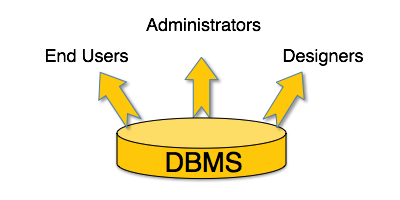
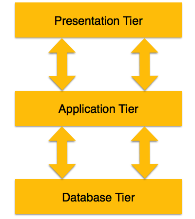
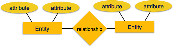
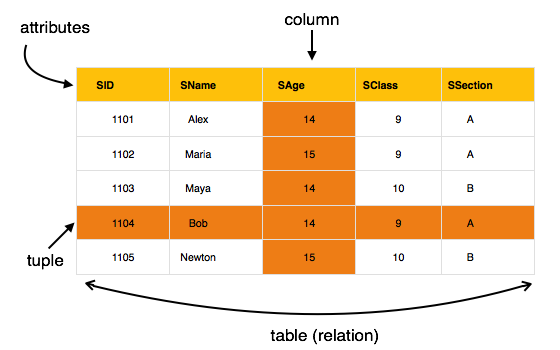
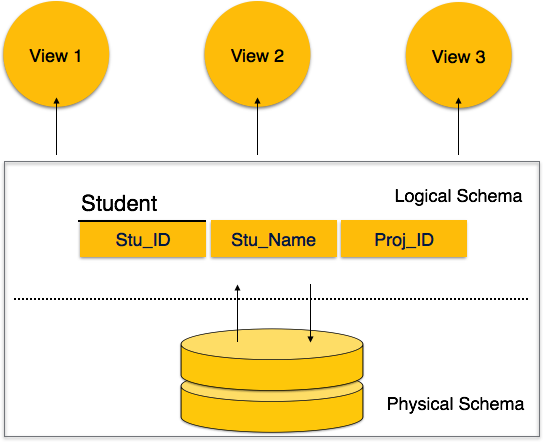
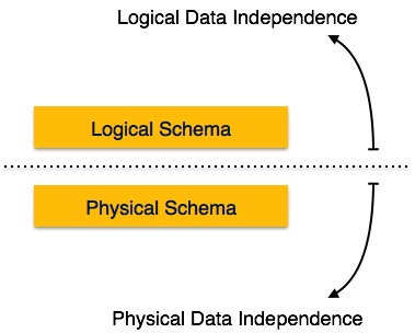


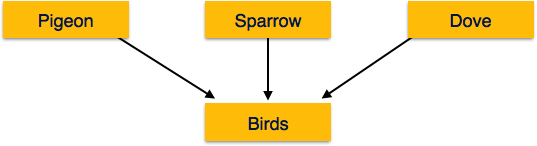
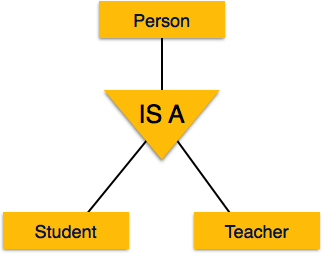
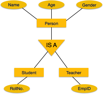
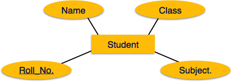
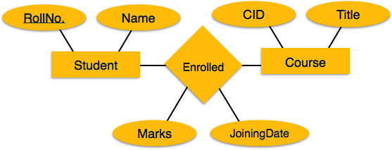
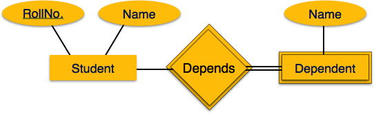
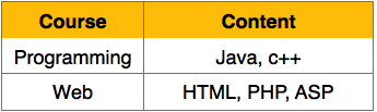
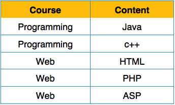
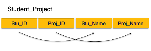
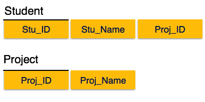
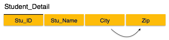
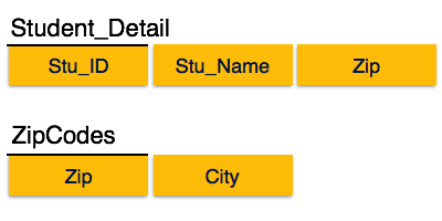
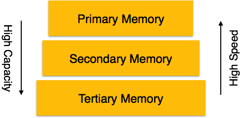
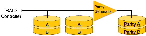
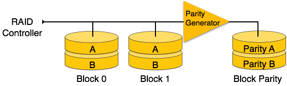
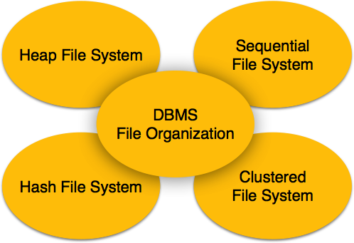
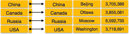
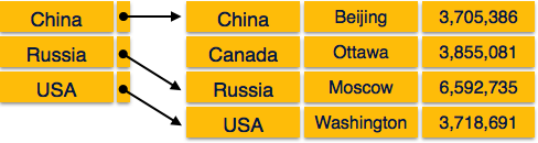
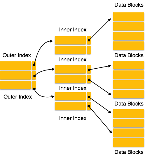
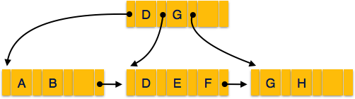
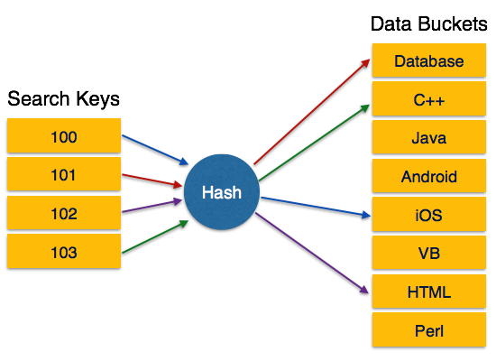
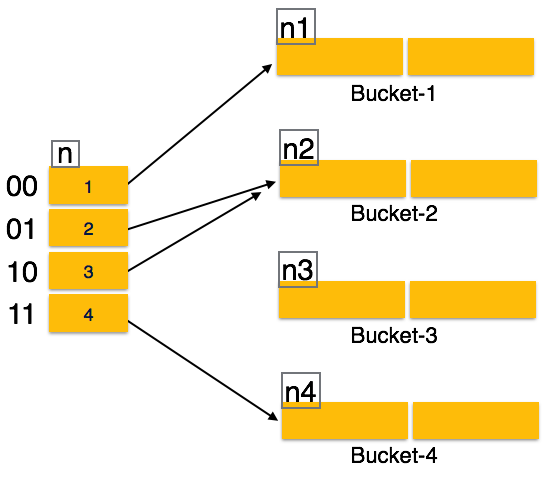
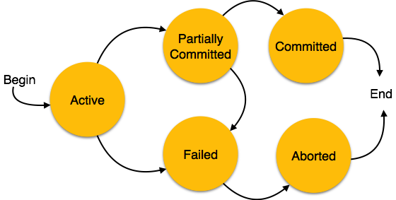
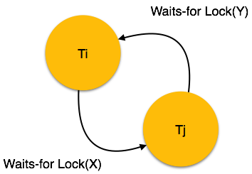
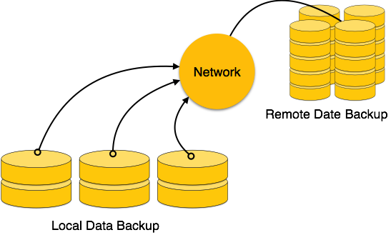
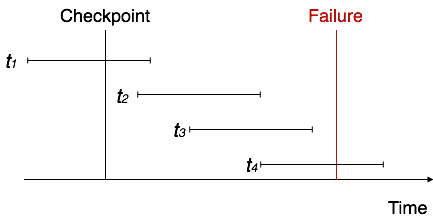
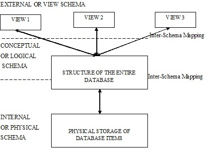

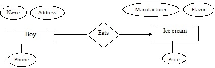


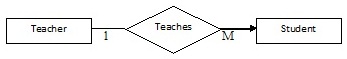

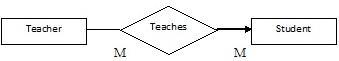


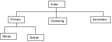
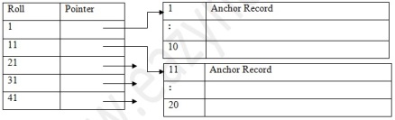
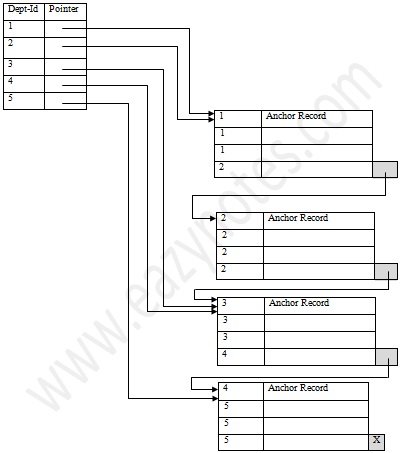
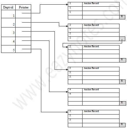
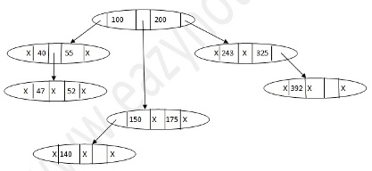
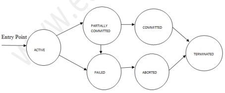
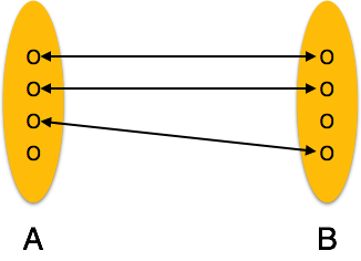
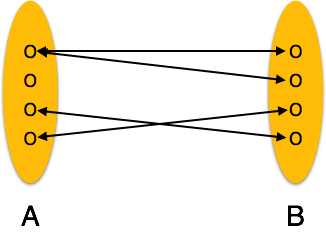
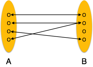
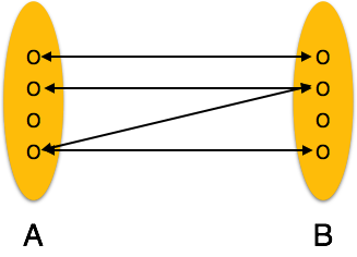


 S )
S ) S )
S ) S)
S)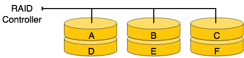
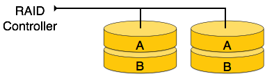
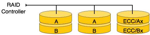
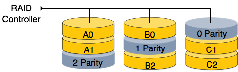
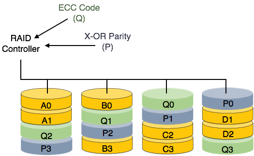
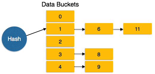
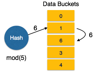


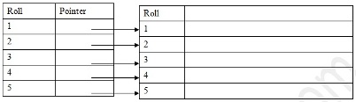
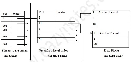


No comments:
Post a Comment